Family Objects

All family objects of the gamlss.dist package, see Rigby et al. (2019), can be used for modelling in gamlss2. However, for users wanting to specify their own (new) distribution model, this document provides a guide on how to define custom family objects within the gamlss2 framework.

Family objects in the gamlss2 package play an essential role in defining the models used for fitting data to distributions. These objects encapsulate the necessary details about the distribution and the parameters, such as:

• The names of the parameters.
• The link functions that map the parameters to the predictor.
• Functions for the density, log-likelihood, and their derivatives.

This document provides an overview of how to construct and use family objects within gamlss2. By the end, you should have a good understanding of how to implement a custom family for use in statistical models.

1 Defining Family Objects

A family object in gamlss2 is a list that must meet the following minimum criteria:

• Family Name: The object must contain the family name as a character string.
• Parameters: The object must list the parameters of the distribution (e.g., "mu" and "sigma" for a normal distribution).
• Link Functions: It must specify the link functions associated with each parameter.
• Probability Density Function: A pdf() function must be provided to evaluate the (log-)density of the distribution.

Optionally, a family object can include functions to calculate the log-likelihood, random number generation, cumulative distribution function (CDF), and quantile function.

Here’s an example of a minimal family object for the normal distribution.

Normal <- function(...) {
  fam <- list(
    "family" = "Normal",
    "names" = c("mu", "sigma"),
    "links" = c("mu" = "identity", "sigma" = "log"),
    "pdf" = function(y, par, log = FALSE, ...) {
      dnorm(y, mean = par$mu, sd = par$sigma, log = log)
    },
    "type" = "continuous"
  )
  class(fam) <- "gamlss2.family"
  return(fam)
}

In this example, we define a normal distribution with two parameters: "mu" (mean) and "sigma" (standard deviation). The link function for "mu" is the identity, and for "sigma", it is the log function. The probability density function (pdf()) must accept the following arguments:

pdf(y, par, log = FALSE, ...)

• y: The response variable.
• par: A named list of parameters (e.g., "mu", "sigma" for the normal distribution).
• log: A logical value indicating whether to return the log-density.

Here, the pdf() function uses the standard dnorm() function to calculate the normal density.

2 Optional Derivatives

Family objects can optionally include functions to compute the first and second derivatives of the log-likelihood with respect to the predictors (or the expected values of those derivatives). These functions are used during model fitting to improve optimization efficiency and accuracy.

All derivative functions must follow the structure:

function(y, par, ...)

First-order derivatives must be provided as a named list called "score", with one function per distribution parameter. Second-order derivatives must be provided in a list named "hess". Each function in "hess" must return the negative (expected) second derivative with respect to the predictor.

The following code illustrates how to provide both "score" and "hess" functions for a normal distribution:

Normal <- function(...) {
  fam <- list(
    "family" = "Normal",
    "names" = c("mu", "sigma"),
    "links" = c("mu" = "identity", "sigma" = "log"),
    "pdf" = function(y, par, log = FALSE, ...) {
      dnorm(y, mean = par$mu, sd = par$sigma, log = log)
    },
    "type" = "continuous",
    "initialize" = list(
      "mu"    = function(y, ...) { (y + mean(y)) / 2 },
      "sigma" = function(y, ...) { rep(sd(y), length(y)) }
    ),
    "score" = list(
      "mu" = function(y, par, ...) {
        (y - par$mu) / (par$sigma^2)
      },
      "sigma" = function(y, par, ...) {
        -1 + (y - par$mu)^2 / (par$sigma^2)
      }
    ),
    "hess" = list(
      "mu" = function(y, par, ...) {
        1 / (par$sigma^2)
      },
      "sigma" = function(y, par, ...) {
        rep(2, length(y))
      },
      "mu.sigma" = function(y, par, ...) {
        rep(0, length(y)) ## example cross-derivative
      }
    )
  )
  class(fam) <- "gamlss2.family"
  return(fam)
}

If no derivative functions are provided, all necessary derivatives will be approximated numerically. In addition to derivatives with respect to single parameters, cross-derivatives (i.e., second-order derivatives involving two different parameters) can also be specified. These should be added to the "hess" list and named using the format "param1.param2", for example "mu.sigma". They must use the same function arguments as the other derivative functions.

Cross-derivatives can be beneficial when using second-order optimization algorithms such as Cole and Green (CG) flavor implemented in the default backfitting algorithm RS in gamlss2. Supplying analytical expressions for these derivatives can significantly improve convergence speed and numerical stability in such settings.

Note that the family object may also include a list of initialization functions for the model parameters. Providing suitable starting values can significantly improve the stability and speed of the estimation process.

3 Additional Functions

Family objects can also include other functions such as

• cdf(y, par, ...): Cumulative distribution function.
• quantile(p, par, ...): Quantile function with probability vector p.
• random(n, par, ...): Random number generation with number of samples n.
• mean(par, ...): Mean function.
• variance(par, ...): Variance function.
• skewness(par, ...): Skewness function.
• kurtosis(par, ...): Kurtosis function.
• valid.response(y): Function to check the values of the response.

Note that the cdf() function is needed it for computing the quantile residuals.

A complete version of the Normal() family is given below:

Normal <- function(...) {
  fam <- list(
    "family" = "Normal",
    "names" = c("mu", "sigma"),
    "links" = c("mu" = "identity", "sigma" = "log"),
    "pdf" = function(y, par, log = FALSE, ...) {
      dnorm(y, mean = par$mu, sd = par$sigma, log = log)
    },
    "cdf" = function(y, par, ...) {
      pnorm(y, mean = par$mu, sd = par$sigma, ...)
    },
    "random" = function(n, par) {
      rnorm(n, mean = par$mu, sd = par$sigma)
    },
    "quantile" = function(p, par) {
      qnorm(p, mean = par$mu, sd = par$sigma)
    },
    "mean" = function(par) { par$mu },
    "variance"  = function(par) { par$sigma^2 },
    "skewness" = function(par) { rep(0, length(par$mu)) },
    "kurtosis" = function(par) { rep(3, length(par$mu)) },
    "type" = "continuous",
    "initialize" = list(
      "mu"    = function(y, ...) { (y + mean(y)) / 2 },
      "sigma" = function(y, ...) { rep(sd(y), length(y)) }
    ),
    "valid.response" = function(y) {
      if(is.factor(y) | is.character(y))
        stop("the response should be numeric!")
      return(TRUE)
    },
    "score" = list(
      "mu" = function(y, par, ...) {
        (y - par$mu) / (par$sigma^2)
      },
      "sigma" = function(y, par, ...) {
        -1 + (y - par$mu)^2 / (par$sigma^2)
      }
    ),
    "hess" = list(
      "mu" = function(y, par, ...) {
        1 / (par$sigma^2)
      },
      "sigma" = function(y, par, ...) {
        rep(2, length(y))
      },
      "mu.sigma" = function(y, par, ...) {
        rep(0, length(y)) ## example cross-derivative
      }
    )
  )
  class(fam) <- "gamlss2.family"
  return(fam)
}

4 Flexible Links

The example above used static link functions to define the family object. However, gamlss2 also allows users to define families with flexible link functions. To support this, the helper function make.link2() is used. The only nontrivial part is adapting the score and hess functions to work on the linear predictor scale. This is not done automatically in gamlss2 for performance reasons - users may even write these functions in C for speed. Below is a minimal example of implementing the Normal family with flexible link functions:

Normal <- function(mu.link = "identity", sigma.link = "log", ...) {
  mu.link <- make.link2(mu.link)
  sigma.link <- make.link2(sigma.link)

  fam <- list(
    "family" = "Normal",
    "names" = c("mu", "sigma"),
    "links" = c("mu" = mu.link, "sigma" = sigma.link),
    "pdf" = function(y, par, log = FALSE, ...) {
      dnorm(y, mean = par$mu, sd = par$sigma, log = log)
    },
    "type" = "continuous"
  )

  class(fam) <- "gamlss2.family"
  return(fam)
}

Note that the score and hess elements are omitted and approximated numerically during estimation.

The following is a small example using the new Normal family with different link functions. We now compare two models, one using an identity link (default) and one using a flexible softplus link.

## load the abdominal circumference data
data("abdom", package = "gamlss.data")
     
## specify the model Formula
f <- y ~ s(x) | s(x)
     
## estimate models
m1 <- gamlss2(f, data = abdom, family = Normal(mu.link = "identity"))

GAMLSS-RS iteration  1: Global Deviance = 4785.931 eps = 0.999867     
GAMLSS-RS iteration  2: Global Deviance = 4785.931 eps = 0.000000     

m2 <- gamlss2(f, data = abdom, family = Normal(mu.link = softplus))

GAMLSS-RS iteration  1: Global Deviance = 4785.931 eps = 0.999866     
GAMLSS-RS iteration  2: Global Deviance = 4785.931 eps = 0.000000     

The fitted means are visualized with

plot(y ~ x, data = abdom, pch = 19,
  col = rgb(0.1, 0.1, 0.1, alpha = 0.3))
lines(abdom$x, mean(m1), col = 2, lwd = 5)
lines(abdom$x, mean(m2), col = 4, lwd = 2)
legend("topleft",
  legend = c("Identity", "Softplus"),
  col = c(2, 4), lwd = 2, bty = "n")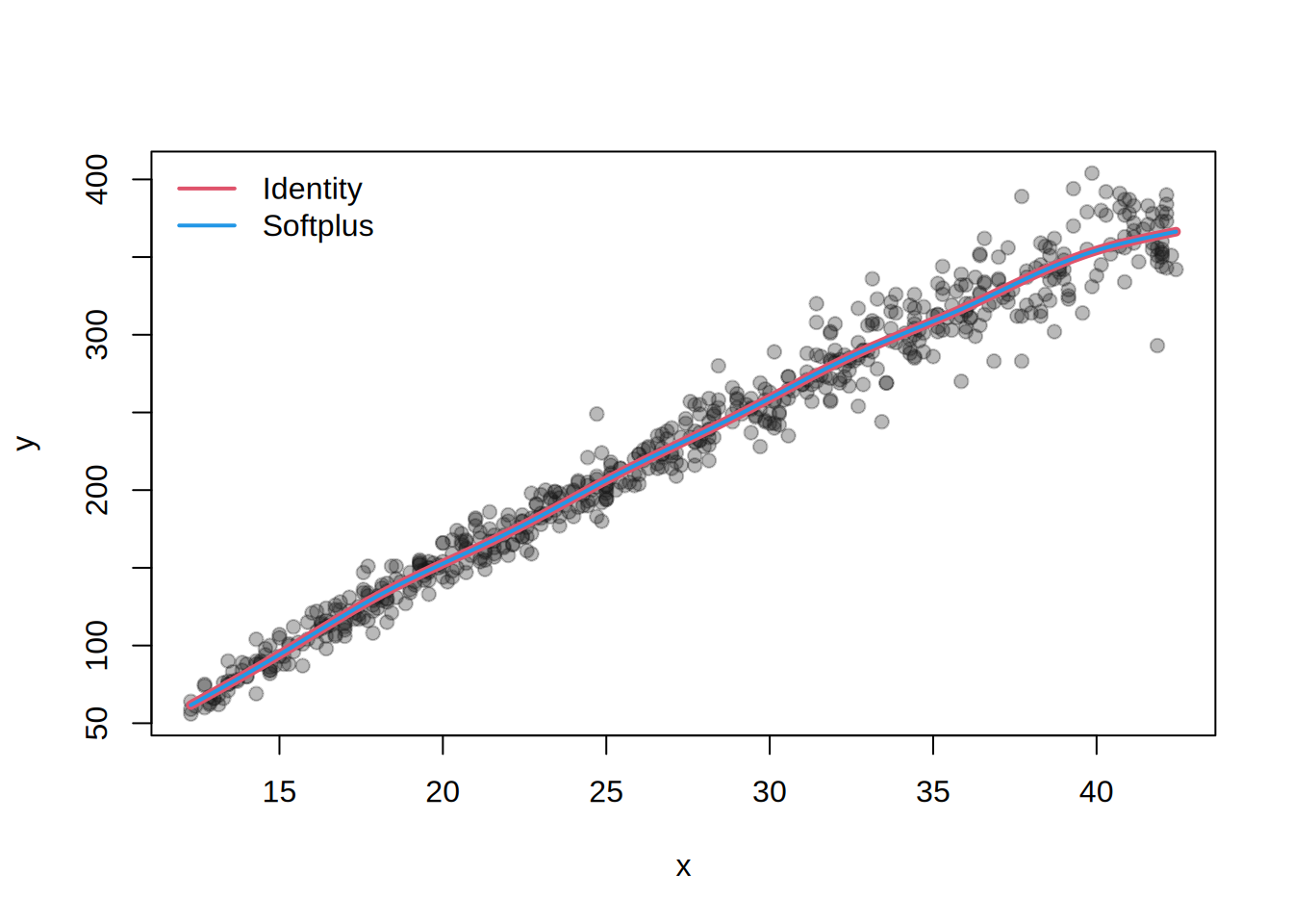

Both models yield identical fits in this case, however, in practice, flexible links can help stabilize estimation or improve fit in more complex scenarios.

5 Summary

Family objects in the gamlss2 package are a fundamental component for defining flexible, distributional regression models, and beyond. By encapsulating the necessary elements, such as parameters, link functions, and probability density functions, they provide a powerful framework for customizing models to fit specific data. The flexibility to define custom families, as demonstrated with the Normal() distribution, enables users to extend the package beyond its default families, making it adaptable to a wide range of modeling scenarios.

References

Rigby, R. A., and D. M. Stasinopoulos. 2005. “Generalized Additive Models for Location, Scale and Shape.” Journal of the Royal Statistical Society C 54 (3): 507–54. https://doi.org/10.1111/j.1467-9876.2005.00510.x.

Rigby, R. A., D. M. Stasinopoulos, G. Z. Heller, and F. De Bastiani. 2019. Distributions for Modeling Location, Scale, and Shape: Using GAMLSS in R. Boca Raton: Chapman & Hall/CRC. https://doi.org/10.1201/9780429298547.