First Steps

The package is designed to follow the workflow of well-established model fitting functions like lm() or glm(), i.e., the step of estimating full distributional regression models is actually not very difficult.

We illustrate how gamlss2 builds on the established gamlss framework by modeling daily maximum temperature (Tmax) at Munich Airport (MUC) to estimate the probability of “heat days” (Tmax \(\geq 30^\circ\text{C}\)). Heat days can have serious impacts by stressing highways and railways, increasing the load on healthcare facilities, and affecting airport operations. Using 30 years of historical Tmax data, we fit a flexible distributional regression model that captures the full conditional distribution of daily temperatures. By evaluating this fitted distribution at the \(30^\circ\text{C}\) threshold, we obtain heat-day probabilities. Required packages can be loaded by

if(!("gamlss" %in% installed.packages())) {
  install.packages("gamlss")
}
library("gamlss")
library("gamlss2")

The data comes from the same R-universe as gamlss2 and is loaded with

if(!("WeatherGermany" %in% installed.packages())) {
  install.packages('WeatherGermany',
    repos = c("https://gamlss-dev.r-universe.dev",
              "https://cloud.r-project.org"))
}

Installing package into '/usr/local/lib/R/site-library'
(as 'lib' is unspecified)

data("WeatherGermany", package = "WeatherGermany")
MUC <- subset(WeatherGermany, id == 1262)

We find that the four-parameter SEP family fits the marginal distribution of Tmax quite well. To estimate a full distributional model, we specify the following additive predictor

\(\eta = \beta_0 + f_1(\texttt{year}) + f_2(\texttt{yday}) + f_3(\texttt{year}, \texttt{yday})\)

for each parameter. Here, \(f_1( \cdot )\) captures the long-term trend, \(f_2( \cdot )\) models seasonal variation, and \(f_3( \cdot, \cdot )\) represents a time-varying seasonal effect. The required variables can be added to the data by

MUC$year <- as.POSIXlt(MUC$date)$year + 1900
MUC$yday <- as.POSIXlt(MUC$date)$yday

In gamlss, model estimation is performed via

if(!("gamlss.add" %in% installed.packages())) {
  install.packages("gamlss.add",
    repos = c("https://gamlss-dev.r-universe.dev",
              "https://cloud.r-project.org"))
}
library("gamlss.add")

f1 <- Tmax ~ ga(~ s(year) + s(yday, bs = "cc") +
  te(year, yday, bs = c("cr", "cc")))
b1 <- gamlss(f1, family = SEP,
  data = MUC[, c("Tmax", "year", "yday")])

GAMLSS-RS iteration 1: Global Deviance = 65081.31 
GAMLSS-RS iteration 2: Global Deviance = 64953.19 
GAMLSS-RS iteration 3: Global Deviance = 64893.26 
GAMLSS-RS iteration 4: Global Deviance = 64869.21 
GAMLSS-RS iteration 5: Global Deviance = 64859.01 
GAMLSS-RS iteration 6: Global Deviance = 64854.42 
GAMLSS-RS iteration 7: Global Deviance = 64852.19 
GAMLSS-RS iteration 8: Global Deviance = 64850.94 
GAMLSS-RS iteration 9: Global Deviance = 64850.14 
GAMLSS-RS iteration 10: Global Deviance = 64849.54 
GAMLSS-RS iteration 11: Global Deviance = 64849.04 
GAMLSS-RS iteration 12: Global Deviance = 64848.58 
GAMLSS-RS iteration 13: Global Deviance = 64848.13 
GAMLSS-RS iteration 14: Global Deviance = 64847.73 
GAMLSS-RS iteration 15: Global Deviance = 64847.33 
GAMLSS-RS iteration 16: Global Deviance = 64846.94 
GAMLSS-RS iteration 17: Global Deviance = 64846.56 
GAMLSS-RS iteration 18: Global Deviance = 64846.19 
GAMLSS-RS iteration 19: Global Deviance = 64845.83 
GAMLSS-RS iteration 20: Global Deviance = 64845.48 

Warning in RS(): Algorithm RS has not yet converged

This setup requires loading the gamlss.add package to access mgcv-based smooth terms. Estimation takes 20 iterations of the backfitting algorithm (without full convergence) and about 44 seconds on a 64-bit Linux system. Moreover, gamlss() requires that the input data contains no NA values. In gamlss2 the model can be specified directly, following mgcv syntax

f2 <- Tmax ~ s(year) + s(yday, bs = "cc") +
  te(year, yday, bs = c("cr", "cc"))
b2 <- gamlss2(f2, family = SEP, data = MUC)

GAMLSS-RS iteration  1: Global Deviance = 65323.9477 eps = 0.572873     
GAMLSS-RS iteration  2: Global Deviance = 64896.9424 eps = 0.006536     
GAMLSS-RS iteration  3: Global Deviance = 64855.9254 eps = 0.000632     
GAMLSS-RS iteration  4: Global Deviance = 64850.95 eps = 0.000076     
GAMLSS-RS iteration  5: Global Deviance = 64849.0477 eps = 0.000029     
GAMLSS-RS iteration  6: Global Deviance = 64847.6498 eps = 0.000021     
GAMLSS-RS iteration  7: Global Deviance = 64846.4455 eps = 0.000018     
GAMLSS-RS iteration  8: Global Deviance = 64845.3635 eps = 0.000016     
GAMLSS-RS iteration  9: Global Deviance = 64844.3787 eps = 0.000015     
GAMLSS-RS iteration 10: Global Deviance = 64843.4798 eps = 0.000013     
GAMLSS-RS iteration 11: Global Deviance = 64842.6571 eps = 0.000012     
GAMLSS-RS iteration 12: Global Deviance = 64841.901 eps = 0.000011     
GAMLSS-RS iteration 13: Global Deviance = 64841.2066 eps = 0.000010     
GAMLSS-RS iteration 14: Global Deviance = 64840.5677 eps = 0.000009     

This model converges in 11 iterations and requires only about 2 seconds of computation time, yielding a similar deviance (small differences arise due to differences in smoothing parameter optimization). In many applications, it is desirable to use the same predictor structure for all distribution parameters. In gamlss, this requires specifying identical formulas separately via sigma.formula, nu.formula, and tau.formula, which can be tedious. In gamlss2, this is simplified using “.”

f3 <- Tmax ~ s(year) + s(yday, bs = "cc") +
  te(year, yday, bs = c("cr", "cc")) | . | . | .
b3 <- gamlss2(f3, family = SEP, data = MUC)

GAMLSS-RS iteration  1: Global Deviance = 64645.6379 eps = 0.577308     
GAMLSS-RS iteration  2: Global Deviance = 64595.3869 eps = 0.000777     
GAMLSS-RS iteration  3: Global Deviance = 64588.1638 eps = 0.000111     
GAMLSS-RS iteration  4: Global Deviance = 64585.17 eps = 0.000046     
GAMLSS-RS iteration  5: Global Deviance = 64582.8773 eps = 0.000035     
GAMLSS-RS iteration  6: Global Deviance = 64580.8716 eps = 0.000031     
GAMLSS-RS iteration  7: Global Deviance = 64579.0939 eps = 0.000027     
GAMLSS-RS iteration  8: Global Deviance = 64577.6793 eps = 0.000021     
GAMLSS-RS iteration  9: Global Deviance = 64576.3714 eps = 0.000020     
GAMLSS-RS iteration 10: Global Deviance = 64575.2258 eps = 0.000017     
GAMLSS-RS iteration 11: Global Deviance = 64574.2289 eps = 0.000015     
GAMLSS-RS iteration 12: Global Deviance = 64573.4533 eps = 0.000012     
GAMLSS-RS iteration 13: Global Deviance = 64572.7665 eps = 0.000010     
GAMLSS-RS iteration 14: Global Deviance = 64572.1738 eps = 0.000009     

This model converges in 20 iterations in about 30 seconds. After estimation, results can be inspected using the summary() method for both packages. Using plot() in gamlss produces standard residual diagnostic plots, whereas in gamlss2

plot(b3)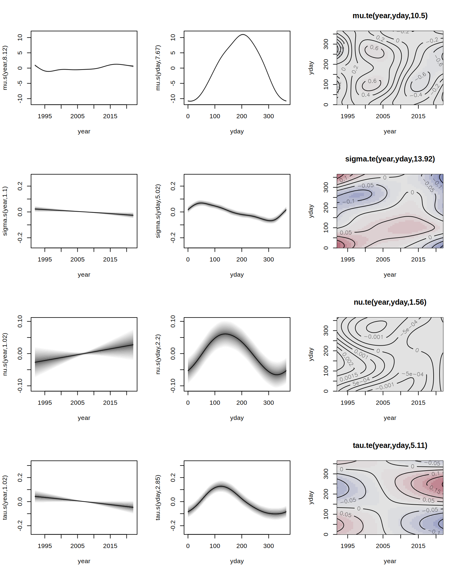

displays all estimated covariate effects. For residual diagnostics, gamlss2 leverages the topmodels package, which provides infrastructures for probabilistic model assessment. E.g., a PIT histogram can be created by

if(!("topmodels" %in% installed.packages())) {
  install.packages("topmodels", repos = "https://zeileis.R-universe.dev")
}
library("topmodels")

pithist(b3)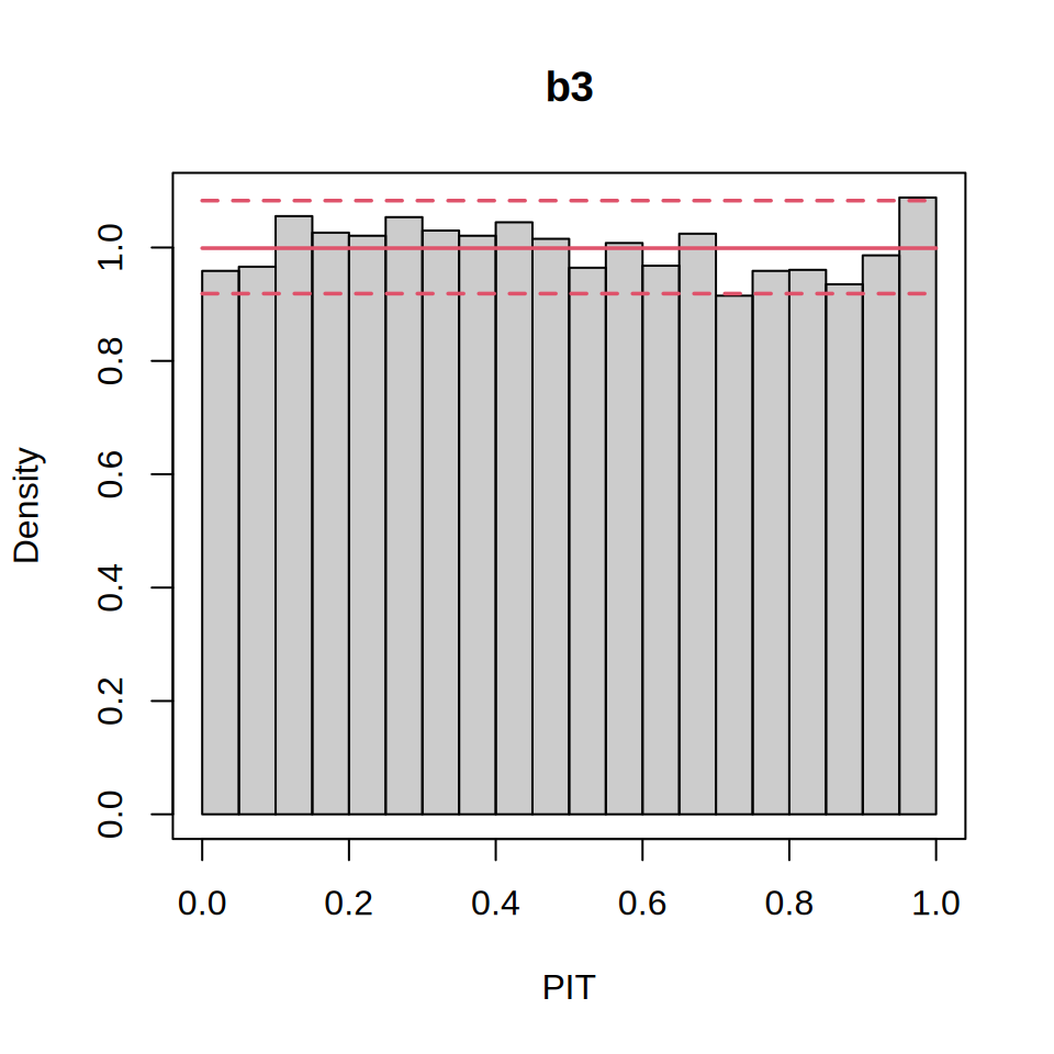

showing good model calibration. Finally, we compute the probability of a heat day for 2025. First, the procast() function from `topmodels predicts the fitted distributions

nd <- data.frame("year" = 2025, "yday" = 0:365)
pf <- procast(b3, newdata = nd, drop = TRUE)

This yields a distribution vector pf using the infrastructure from the distributions3 package. Probabilities of a heat day can then be calculated with the corresponding cdf() method.

if(!("distributions3" %in% installed.packages())) {
  install.packages("distributions3")
}
library("distributions3")
probs <- 1 - cdf(pf, 30)

and visualized, for example, by

par(mar = c(4, 4, 1, 1))
plot(probs, type = "l", xlab = "Day of Year",
  ylab = "Prob(Tmax > 30)")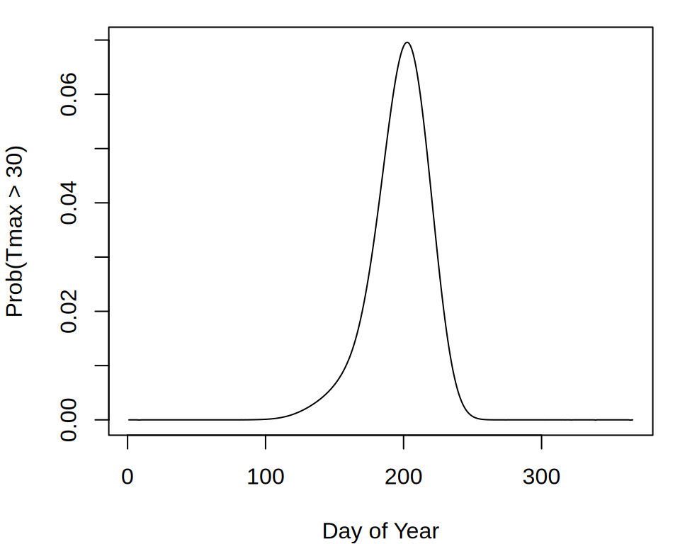

Note that a predict() method is available for both gamlss and gamlss2, allowing direct prediction of distribution parameters. However, in gamlss, predict() may not fully support new data in all cases.

References

Rigby, R. A., and D. M. Stasinopoulos. 2005. “Generalized Additive Models for Location, Scale and Shape.” Journal of the Royal Statistical Society C 54 (3): 507–54. https://doi.org/10.1111/j.1467-9876.2005.00510.x.