library("gamlss2")

## seasonal variation of motorcycle counts at Sonnenberg/Harz
data("HarzTraffic", package = "gamlss2")
plot(bikes ~ yday, data = HarzTraffic)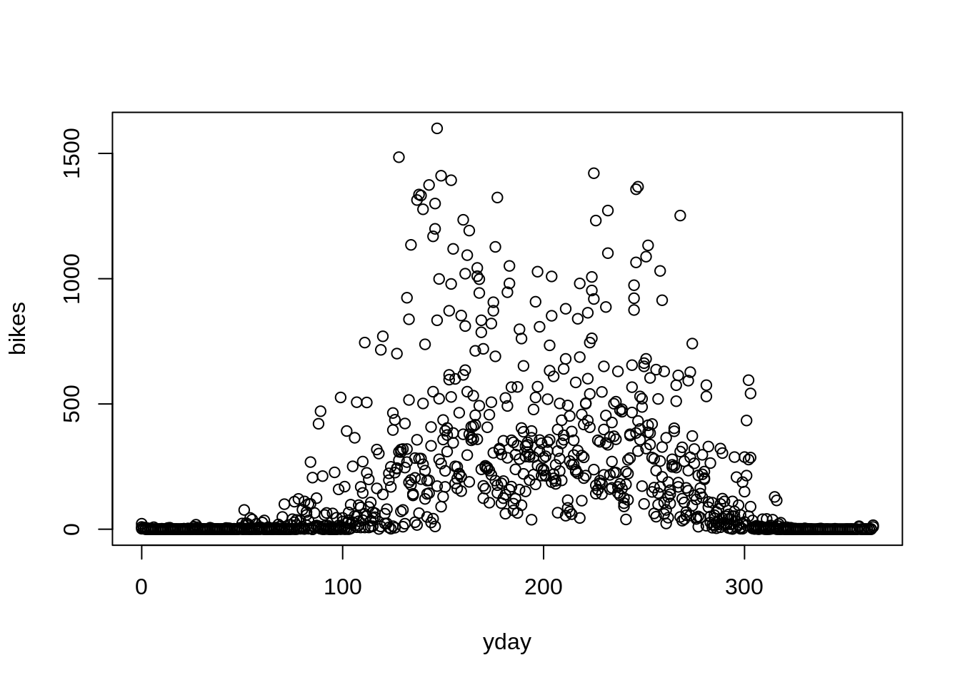
## count distribution
barplot(table(HarzTraffic$bikes))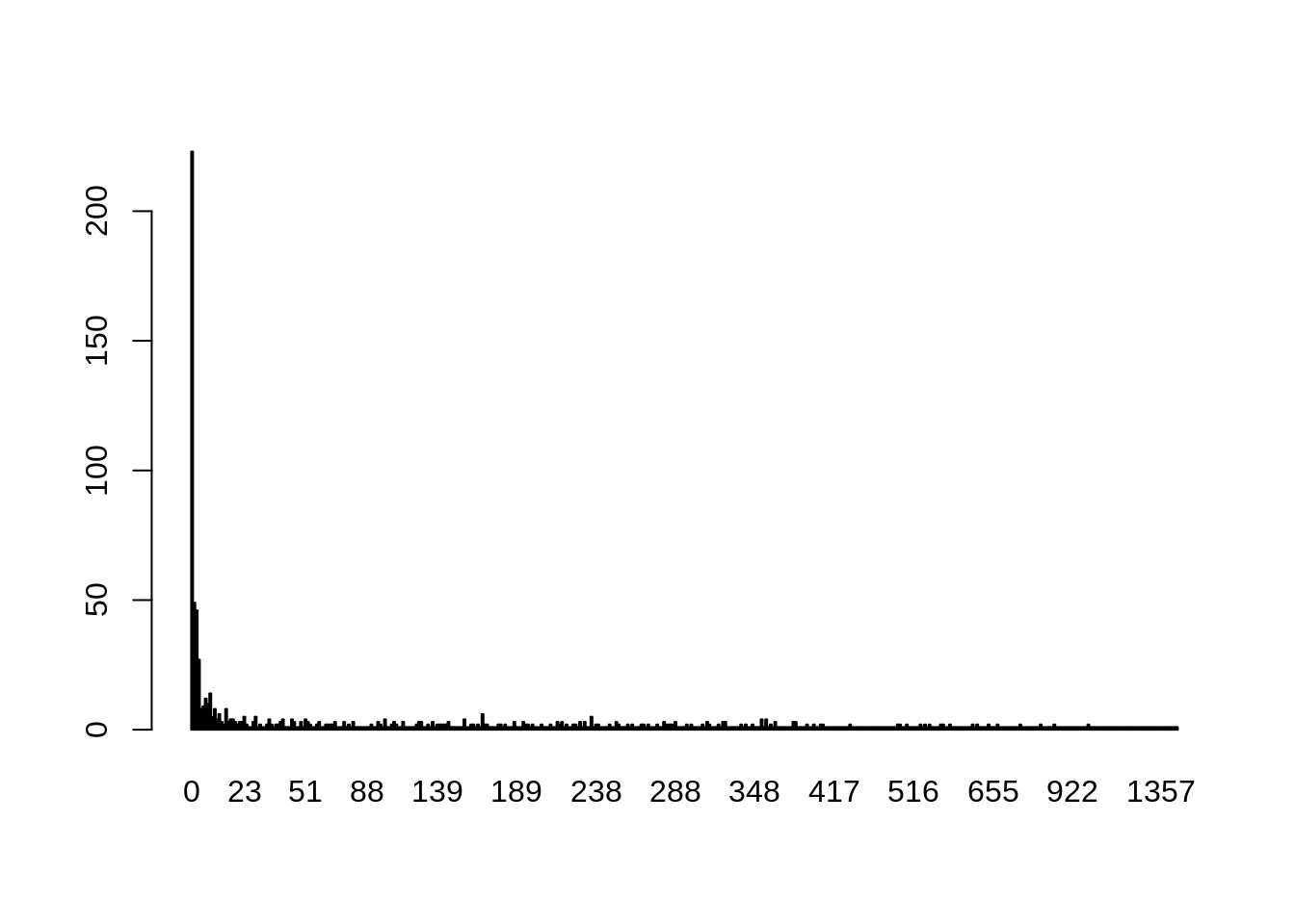
## negative binomial seasonal model using cyclic splines
m <- gamlss2(bikes ~ s(yday, bs = "cc") | s(yday, bs = "cc"),
  data = HarzTraffic, family = NBI)
GAMLSS-RS iteration 1: Global Deviance = 10151.1432 eps = 0.149402
GAMLSS-RS iteration 2: Global Deviance = 10150.8948 eps = 0.000024
GAMLSS-RS iteration 3: Global Deviance = 10150.8818 eps = 0.000001 ## visualize effects
plot(m)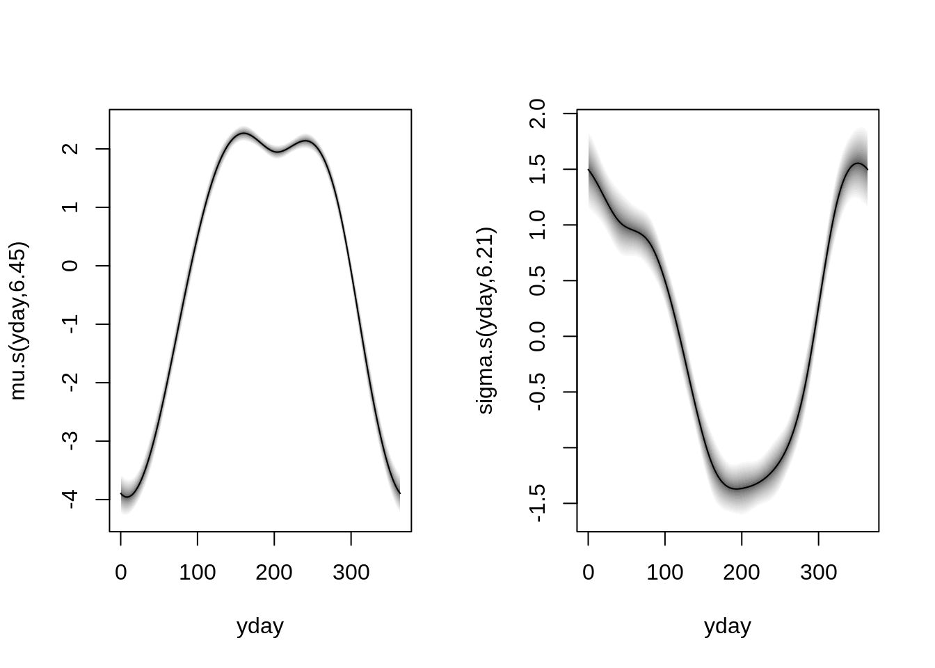
## residual diagnostics
plot(m, which = "resid")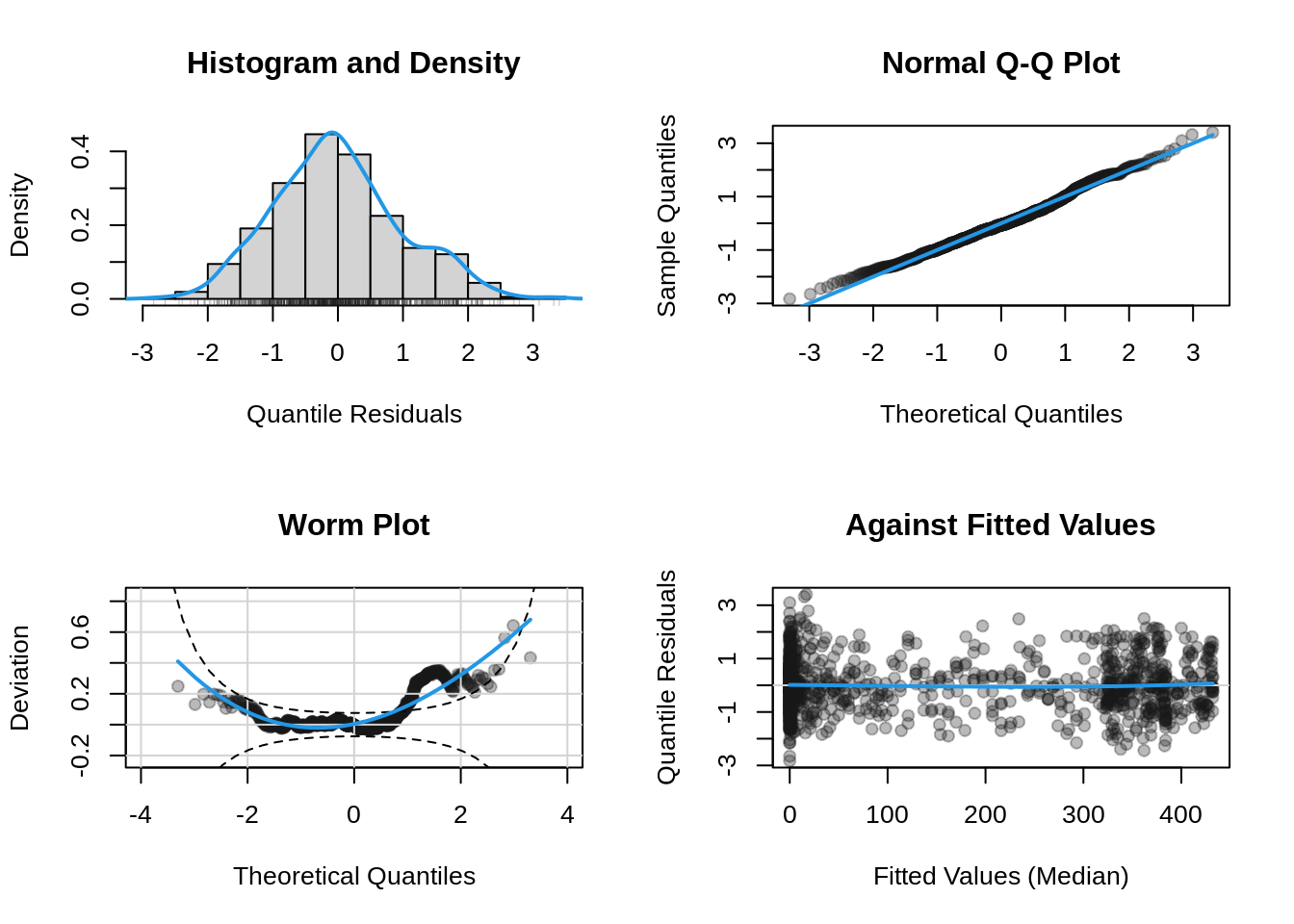
## fitted parameters for each day of the year
nd <- data.frame(yday = 1:365)
## corresponding quantiles
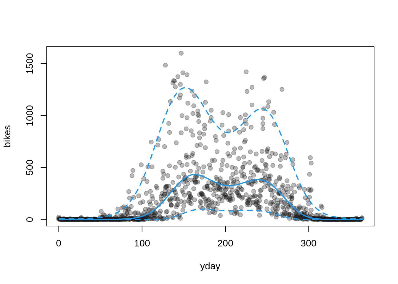
p <- quantile(m, newdata = nd, probs = c(0.05, 0.5, 0.95))
## visualization
plot(bikes ~ yday, data = HarzTraffic, pch = 19, col = gray(0.1, alpha = 0.3))
matlines(nd$yday, p, lty = c(2, 1, 2), lwd = 2, col = 4)