GAIC and Generalised (Pseudo) R-squared for GAMLSS Models

Description

Functions to compute the GAIC and the generalised R-squared of Nagelkerke (1991) for a GAMLSS models.

Usage

## Information criteria.
GAIC(object, ...,
  k = 2, corrected = FALSE)

## R-squared.
Rsq(object, ...,
  type = c("Cox Snell", "Cragg Uhler", "both", "simple"),
  newdata = NULL)

Arguments

object	A fitted model object
…	Optionally more fitted model objects.
k	Numeric, the penalty to be used. The default k = 2 corresponds to the classical AIC.
corrected	Logical, whether the corrected AIC should be used? Note that it applies only when k = 2.
type	which definition of R squared. Can be the “Cox Snell” or the Nagelkerke, “Cragg Uhler” or “both”, and “simple”, which computes the R-squared based on the median. In this case also newdata may be supplied.
newdata	Only for type = “simple” the R-squared can be evaluated using newdata.

Details

The Rsq() function uses the definition for R-squared:

\(R^2=1- \left(\frac{L(0)}{L(\hat{\theta})}\right)^{2/n}\)

where \(L(0)\) is the null model (only a constant is fitted to all parameters) and \(L(\hat{\theta})\) is the current fitted model. This definition sometimes is referred to as the Cox & Snell R-squared. The Nagelkerke /Cragg & Uhler’s definition divides the above with

\(1 - L(0)^{2/n}\)

Value

Numeric vector or data frame, depending on the number of fitted model objects.

References

Nagelkerke NJD (1991). “A Note on a General Definition of the Coefficient of Determination.” Biometrika, 78(3), 691–692. doi:10.1093/biomet/78.3.691

See Also

gamlss2

Examples

library("gamlss2")


## load the aids data set
data("aids", package = "gamlss.data")

## estimate negative binomial count models
b1 <- gamlss2(y ~ x + qrt, data = aids, family = NBI)

GAMLSS-RS iteration  1: Global Deviance = 492.6373 eps = 0.148669     
GAMLSS-RS iteration  2: Global Deviance = 492.6373 eps = 0.000000     

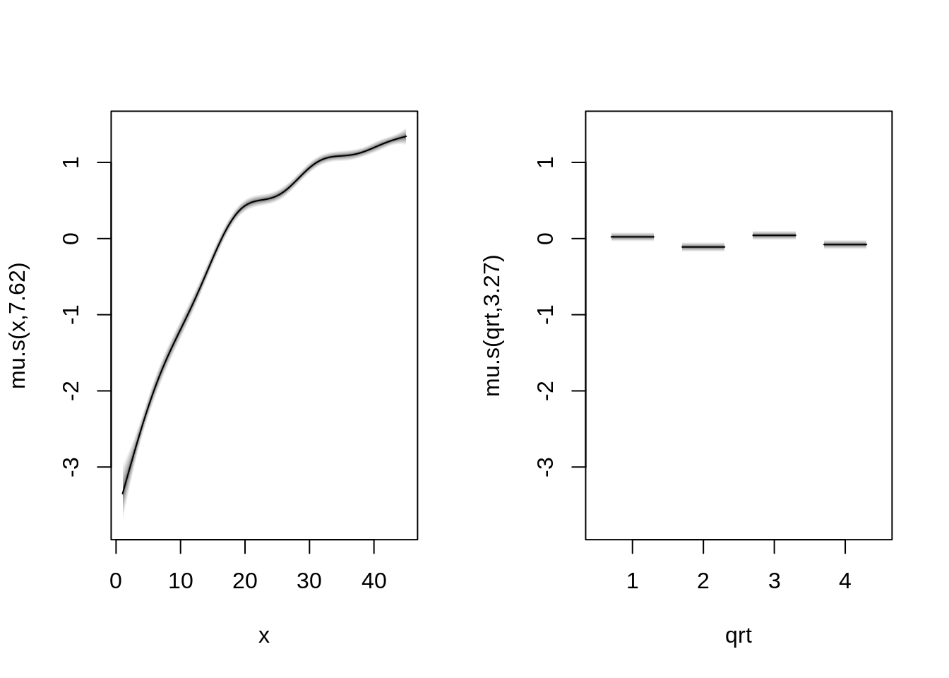
b2 <- gamlss2(y ~ s(x) + s(qrt, bs = "re"), data = aids, family = NBI)

GAMLSS-RS iteration  1: Global Deviance = 365.9324 eps = 0.367629     
GAMLSS-RS iteration  2: Global Deviance = 365.6841 eps = 0.000678     
GAMLSS-RS iteration  3: Global Deviance = 365.6735 eps = 0.000029     
GAMLSS-RS iteration  4: Global Deviance = 365.6634 eps = 0.000027     
GAMLSS-RS iteration  5: Global Deviance = 365.6538 eps = 0.000026     
GAMLSS-RS iteration  6: Global Deviance = 365.6447 eps = 0.000024     
GAMLSS-RS iteration  7: Global Deviance = 365.636 eps = 0.000023     
GAMLSS-RS iteration  8: Global Deviance = 365.6278 eps = 0.000022     
GAMLSS-RS iteration  9: Global Deviance = 365.6199 eps = 0.000021     
GAMLSS-RS iteration 10: Global Deviance = 365.6124 eps = 0.000020     
GAMLSS-RS iteration 11: Global Deviance = 365.6053 eps = 0.000019     
GAMLSS-RS iteration 12: Global Deviance = 365.5986 eps = 0.000018     
GAMLSS-RS iteration 13: Global Deviance = 365.5921 eps = 0.000017     
GAMLSS-RS iteration 14: Global Deviance = 365.586 eps = 0.000016     
GAMLSS-RS iteration 15: Global Deviance = 365.5802 eps = 0.000015     
GAMLSS-RS iteration 16: Global Deviance = 365.5746 eps = 0.000015     
GAMLSS-RS iteration 17: Global Deviance = 365.5693 eps = 0.000014     
GAMLSS-RS iteration 18: Global Deviance = 365.5643 eps = 0.000013     
GAMLSS-RS iteration 19: Global Deviance = 365.5595 eps = 0.000013     
GAMLSS-RS iteration 20: Global Deviance = 365.5549 eps = 0.000012     

## compare models
Rsq(b1)

[1] 0.8095853

Rsq(b1, type = "both")

$CoxSnell
[1] 0.8095853

$CraggUhler
[1] 0.809588

Rsq(b1, b2)

       b1        b2 
0.8095853 0.9886961 

GAIC(b1, b2)

        AIC       df
b2 391.0332 12.73917
b1 504.6373  6.00000

AIC(b1, b2)

        AIC       df
b2 391.0332 12.73917
b1 504.6373  6.00000

BIC(b1, b2)

        AIC       df
b2 414.0486 12.73917
b1 515.4773  6.00000

## plot estimated effects
plot(b2)