Generalized Additive Models for Location Scale and Shape

Description

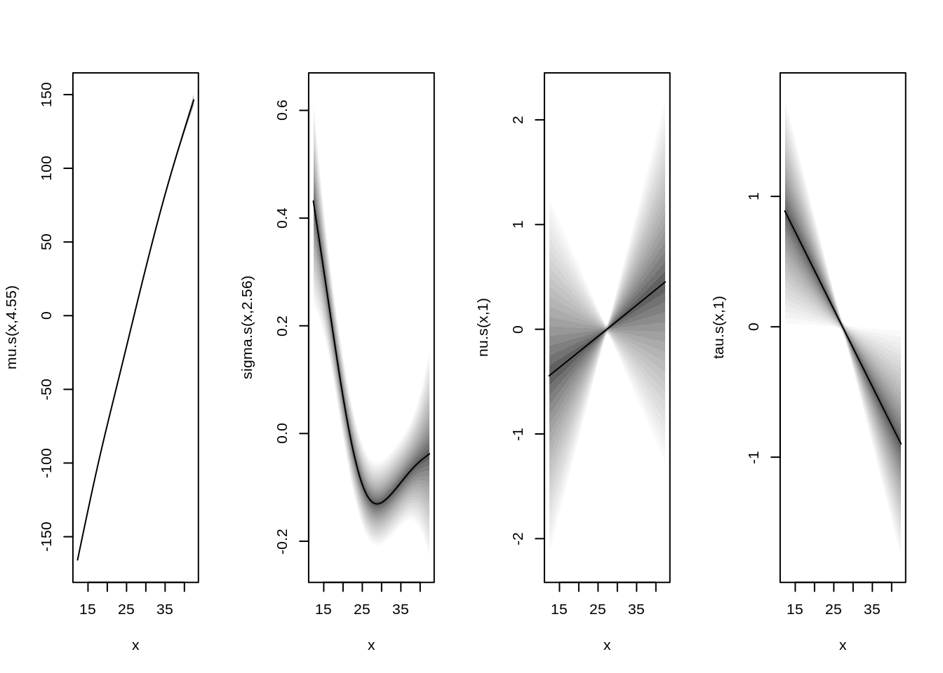
Estimation of generalized additive models for location scale and shape (GAMLSS). The model fitting function gamlss2() provides flexible infrastructures to estimate the parameters of a response distribution. The number of distributional parameters is not fixed, see gamlss2.family. Moreover, gamlss2() supports all smooth term constructors from the mgcv package in addition to the classical model terms as provided by gamlss and gamlss.add.

Usage

gamlss2(x, ...)

## S3 method for class 'formula'
gamlss2(formula, data, family = NO,
  subset, na.action, weights, offset, start = NULL,
  control = gamlss2_control(...), ...)

## S3 method for class 'list'
gamlss2(x, ...)

Arguments

formula	A GAM-type formula or Formula. All smooth terms of the mgcv package are supported, see also formula.gam.
x	For gamlss.list() x is a list of formulas.
data	A data frame or list or environment containing the variables in the model. If not found in data, the variables are taken from environment(formula), typically the environment from which gamlss2 is called.
family	A gamlss.family or gamlss2.family object used to define distribution and the link functions of the parameters.
subset	An optional vector specifying a subset of observations to be used in the fitting process.
na.action	NA processing for setting up the model.frame.
weights	An optional vector of prior weights to be used in the fitting process. Should be NULL or a numeric vector.
offset	This can be used to specify an a priori known components to be included in the linear predictors during fitting. Please note that if only a single numeric vector is provided, the offset will be assigned to the first specified parameter of the distribution. In the case of multiple offsets, a data frame or list must be supplied. Each offset is assigned in the same order as the parameters of the distribution specified in the family object.
start	Starting values for estimation algorithms.
control	A list of control arguments, see gamlss2_control.
…	Arguments passed to gamlss2_control.

Details

The model fitting function gamlss2() provides flexible infrastructures for the estimation of GAMLSS.

• Distributional models are specified using family objects, either from the gamlss.dist package or using gamlss2.family objects.

• Estimation is carried out through a Newton-Raphson/Fisher scoring algorithm, see function RS. The estimation algorithms can also be exchanged using gamlss2_control. Additionally, if an optimizer is specified by the family object, this optimizer function will be employed for estimation.

• The return value is determined by the object returned from the optimizer function, typically an object of class “gamlss2”. Default methods and extractor functions are available for this class. Nevertheless, users have the flexibility to supply their own optimizer function, along with user-specific methods tailored for the returned object.

Value

The return value is determined by the object returned from the optimizer function. By default, the optimization is performed using the RS optimizer function (see gamlss2_control), yielding an object of class “gamlss2”. Default methods and extractor functions are available for this class.

References

Rigby RA, Stasinopoulos DM (2005). “Generalized Additive Models for Location, Scale and Shape (with Discussion).” Journal of the Royal Statistical Society, Series C (Applied Statistics), 54, 507–554. doi:10.1111/j.1467-9876.2005.00510.x

Rigby RA, Stasinopoulos DM, Heller GZ, De Bastiani F (2019). Distributions for Modeling Location, Scale, and Shape: Using GAMLSS in R, Chapman and Hall/CRC. doi:10.1201/9780429298547

Stasinopoulos DM, Rigby RA (2007). “Generalized Additive Models for Location Scale and Shape (GAMLSS) in R.” Journal of Statistical Software, 23(7), 1–46. doi:10.18637/jss.v023.i07

Stasinopoulos DM, Rigby RA, Heller GZ, Voudouris V, De Bastiani F (2017). Flexible Regression and Smoothing: Using GAMLSS in R, Chapman and Hall/CRC. doi:10.1201/b21973

See Also

RS, gamlss2_control, gamlss2.family

Examples

library("gamlss2")


## load the abdominal circumference data
data("abdom", package = "gamlss.data")

## specify the model Formula
f <- y ~ s(x) | s(x) | s(x) | s(x)

## estimate model
b <- gamlss2(f, data = abdom, family = BCT)

GAMLSS-RS iteration  1: Global Deviance = 4774.4683 eps = 0.534345     
GAMLSS-RS iteration  2: Global Deviance = 4770.229 eps = 0.000887     
GAMLSS-RS iteration  3: Global Deviance = 4770.1663 eps = 0.000013     
GAMLSS-RS iteration  4: Global Deviance = 4770.1554 eps = 0.000002     

## model summary
summary(b)

Call:
gamlss2(formula = f, data = abdom, family = BCT)
---
Family: BCT 
Link function: mu = identity, sigma = log, nu = identity, tau = log
*--------
Parameter: mu 
---
Coefficients:
            Estimate Std. Error t value Pr(>|t|)    
(Intercept)  226.334      1.257     180   <2e-16 ***
---
Smooth terms:
     s(x)
edf 4.551
*--------
Parameter: sigma 
---
Coefficients:
            Estimate Std. Error t value Pr(>|t|)    
(Intercept) -2.92264    0.01101  -265.5   <2e-16 ***
---
Smooth terms:
      s(x)
edf 2.5639
*--------
Parameter: nu 
---
Coefficients:
            Estimate Std. Error t value Pr(>|t|)    
(Intercept) -0.18021    0.04599  -3.918 9.95e-05 ***
---
Smooth terms:
      s(x)
edf 1.0015
*--------
Parameter: tau 
---
Coefficients:
            Estimate Std. Error t value Pr(>|t|)    
(Intercept)   2.6548     0.0144   184.4   <2e-16 ***
---
Signif. codes:  0 '***' 0.001 '**' 0.01 '*' 0.05 '.' 0.1 ' ' 1
---
Smooth terms:
      s(x)
edf 1.0042
*--------
n = 610 df =  13.12 res.df =  596.88
Deviance = 4770.1554 Null Dev. Red. = 33.39%
AIC = 4796.3966 elapsed =  0.78sec

## plot estimated effects
plot(b, which = "effects")

## plot diagnostics
plot(b, which = "resid")

## predict parameters
par <- predict(b)

## predict quantiles
pq <- sapply(c(0.05, 0.5, 0.95), function(q) family(b)$q(q, par))

## visualize
plot(y ~ x, data = abdom, pch = 19,
  col = rgb(0.1, 0.1, 0.1, alpha = 0.3))
matplot(abdom$x, pq, type = "l", lwd = 2,
  lty = 1, col = 4, add = TRUE)

## use of starting values
m <- gamlss2(f, data = abdom, family = BCT,
  start = c(mu = 200, sigma = 0.1, nu = 0, tau = 10))

GAMLSS-RS iteration  1: Global Deviance = 4789.7797 eps = 0.556012     
GAMLSS-RS iteration  2: Global Deviance = 4774.5657 eps = 0.003176     
GAMLSS-RS iteration  3: Global Deviance = 4771.4193 eps = 0.000658     
GAMLSS-RS iteration  4: Global Deviance = 4769.9947 eps = 0.000298     
GAMLSS-RS iteration  5: Global Deviance = 4769.9556 eps = 0.000008     

## fix some parameters
m <- gamlss2(f, data = abdom, family = BCT,
  start = c(mu = 200, sigma = 0.1, nu = 0, tau = 10),
  fixed = c(nu = TRUE, tau = TRUE))

GAMLSS-RS iteration  1: Global Deviance = 4799.422 eps = 0.555118     
GAMLSS-RS iteration  2: Global Deviance = 4795.2807 eps = 0.000862     
GAMLSS-RS iteration  3: Global Deviance = 4795.2668 eps = 0.000002     

## estimated coefficients (intercepts)
coef(m)

   mu.p.(Intercept) sigma.p.(Intercept)    nu.p.(Intercept)   tau.p.(Intercept) 
         226.347632           -2.922923            0.000000            2.302585 

## starting values using full predictors
m <- gamlss2(f, data = abdom, family = BCT,
  start = fitted(m))

GAMLSS-RS iteration  1: Global Deviance = 4902.0767 eps = 0.372276     
GAMLSS-RS iteration  2: Global Deviance = 4775.8465 eps = 0.025750     
GAMLSS-RS iteration  3: Global Deviance = 4775.0302 eps = 0.000170     
GAMLSS-RS iteration  4: Global Deviance = 4774.9582 eps = 0.000015     
GAMLSS-RS iteration  5: Global Deviance = 4774.9519 eps = 0.000001     

## same with
m <- gamlss2(f, data = abdom, family = BCT,
  start = m)

GAMLSS-RS iteration  1: Global Deviance = 4774.4683 eps = 0.534345     
GAMLSS-RS iteration  2: Global Deviance = 4770.229 eps = 0.000887     
GAMLSS-RS iteration  3: Global Deviance = 4770.1663 eps = 0.000013     
GAMLSS-RS iteration  4: Global Deviance = 4770.1554 eps = 0.000002