prodist.gamlss2 – gamlss2

Extracting Fitted or Predicted Probability Distributions from gamlss2 Models

Description

Methods for gamlss2 model objects for extracting fitted (in-sample) or predicted (out-of-sample) probability distributions as distributions3 objects.

Usage

## S3 method for class 'gamlss2'
prodist(object, ...)

Arguments

`object`	A model object of class `gamlss2`.
`…`	Arguments passed on to `predict.gamlss2`, e.g., `newdata`.

Details

To facilitate making probabilistic forecasts based on gamlss2 model objects, the prodist method extracts fitted or predicted probability distribution objects. Internally, the predict.gamlss2 method is used first to obtain the distribution parameters (mu, sigma, tau, nu, or a subset thereof). Subsequently, the corresponding distribution object is set up using the GAMLSS class from the gamlss.dist package, enabling the workflow provided by the distributions3 package (see Zeileis et al. 2022).

Note that these probability distributions only reflect the random variation in the dependent variable based on the model employed (and its associated distributional assumption for the dependent variable). This does not capture the uncertainty in the parameter estimates.

Value

An object of class GAMLSS inheriting from distribution.

References

Zeileis A, Lang MN, Hayes A (2022). “distributions3: From Basic Probability to Probabilistic Regression.” Presented at useR! 2022 - The R User Conference. Slides, video, vignette, code at https://www.zeileis.org/news/user2022/.

Examples

library("gamlss2")


## packages, code, and data
library("distributions3")
data("cars", package = "datasets")

## fit heteroscedastic normal GAMLSS model
## stopping distance (ft) explained by speed (mph)
m <- gamlss2(dist ~ s(speed) | s(speed), data = cars, family = NO)

GAMLSS-RS iteration  1: Global Deviance = 407.3541 eps = 0.125497     
GAMLSS-RS iteration  2: Global Deviance = 405.7146 eps = 0.004024     
GAMLSS-RS iteration  3: Global Deviance = 405.6978 eps = 0.000041     
GAMLSS-RS iteration  4: Global Deviance = 405.6976 eps = 0.000000

## obtain predicted distributions for three levels of speed
d <- prodist(m, newdata = data.frame(speed = c(10, 20, 30)))
print(d)

                                     1                                      2 
"GAMLSS NO(mu = 23.04, sigma = 10.06)" "GAMLSS NO(mu = 59.04, sigma = 18.51)" 
                                     3 
"GAMLSS NO(mu = 96.35, sigma = 33.95)"

## obtain quantiles (works the same for any distribution object 'd' !)
quantile(d, 0.5)

       1        2        3 
23.03912 59.03607 96.34896

quantile(d, c(0.05, 0.5, 0.95), elementwise = FALSE)

     q_0.05    q_0.5    q_0.95
1  6.486962 23.03912  39.59128
2 28.589641 59.03607  89.48250
3 40.504887 96.34896 152.19303

quantile(d, c(0.05, 0.5, 0.95), elementwise = TRUE)

         1          2          3 
  6.486962  59.036073 152.193030

## visualization
plot(dist ~ speed, data = cars)
nd <- data.frame(speed = 0:240/4)
nd$dist <- prodist(m, newdata = nd)
nd$fit <- quantile(nd$dist, c(0.05, 0.5, 0.95))
matplot(nd$speed, nd$fit, type = "l", lty = 1, col = "slategray", add = TRUE)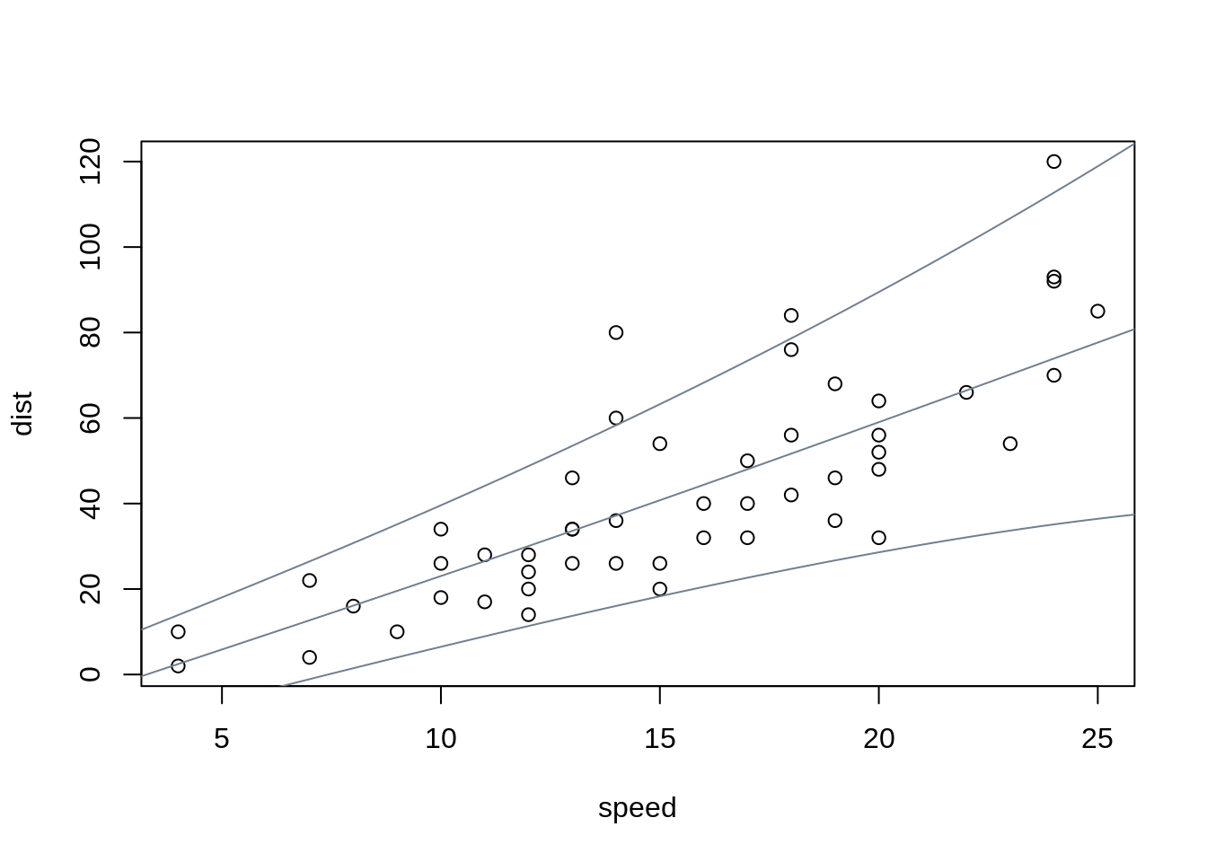

## moments
mean(d)

       1        2        3 
23.03912 59.03607 96.34896

variance(d)

        1         2         3 
 101.2639  342.6244 1152.6558

## simulate random numbers
random(d, 5)

       r_1      r_2       r_3      r_4      r_5
1 33.11540 24.50488  9.441543 25.11586 27.93865
2 59.01081 66.08557 75.755813 35.06851 42.55242
3 85.75660 94.74387 82.995691 99.05468 85.37200

## density and distribution
pdf(d, 50 * -2:2)

        d_-100        d_-50          d_0        d_50        d_100
1 1.365786e-34 1.440750e-13 0.0028836944 0.001095127 7.891037e-15
2 2.012473e-18 6.289547e-10 0.0001332376 0.019131662 1.862073e-03
3 6.414012e-10 1.084300e-06 0.0002095201 0.004627633 1.168286e-02

cdf(d, 50 * -2:2)

        p_-100        p_-50          p_0       p_50     p_100
1 1.116699e-34 1.961566e-13 0.0110254856 0.99631019 1.0000000
2 4.279141e-18 1.923739e-09 0.0007128545 0.31271491 0.9865531
3 3.661574e-09 8.139843e-06 0.0022705648 0.08609812 0.5428194

## Poisson example
data("FIFA2018", package = "distributions3")
m2 <- gamlss2(goals ~ s(difference), data = FIFA2018, family = PO)

GAMLSS-RS iteration  1: Global Deviance = 355.3922 eps = 0.045332     
GAMLSS-RS iteration  2: Global Deviance = 355.3922 eps = 0.000000

d2 <- prodist(m2, newdata = data.frame(difference = 0))
print(d2)

                      1 
"GAMLSS PO(mu = 1.237)"

quantile(d2, c(0.05, 0.5, 0.95))

[1] 0 1 3

## note that log_pdf() can replicate logLik() value
sum(log_pdf(prodist(m2), FIFA2018$goals))

[1] -177.6961

logLik(m2)

'log Lik.' -177.6961 (df=2.005144)