gamlss2

Softplus Link Object

Description

Link object (with link function, inverse link function, etc.) that assures positivity of parameters based on the softplus function.

Usage

softplus(a = 1)

Arguments

a Extra parameter of the generalized softplus function

Details

The softplus link function with parameter \(a\) is given by:

\(\displaystyle \frac{\log(1 + \exp(a \cdot x))}{a}\)

This is an approximation of the linear spline \(\max\{0, x\}\) where the discrepancy between the two functions decreases with increasing \(a\).

Wiemann et al. (2023) propose to employ the softplus function as the inverse link function where positivity of a parameter needs to be assured, e.g., in count data regressions. This is in particular of interest as an alternative to the exponential inverse link function because the exponential implies multiplicative effects of the regressors while the softplus function does not.

Value

An object of class “link-glm”.

References

Wiemann PFV, Kneib T, Hambuckers J (2023). “Using the Softplus Function to Construct Alternative Link Functions in Generalized Linear Models and Beyond.” Statistical Papers, forthcoming. doi:https://doi.org/10.1007/s00362-023-01509-x

Examples

library("gamlss2")


## visualization of softmax function from Wiemann et al. (2003, Figure 1)
x <- -200:200/50
plot(x, softplus(1)$linkinv(x), ylab = expression(softplus[a](x)),
  type = "l", col = 2, lwd = 2)
grid()
lines(x, softplus(5)$linkinv(x), col = 3, lwd = 2)
lines(x, softplus(10)$linkinv(x), col = 4, lwd = 2)
lines(x, pmax(0, x), lty = 3, lwd = 2)
legend("topleft", c("a = 1", "a = 5", "a = 10", "linear spline"),
  col = c(2, 3, 4, 1), lty = c(1, 1, 1, 3), lwd = 2, bty = "n")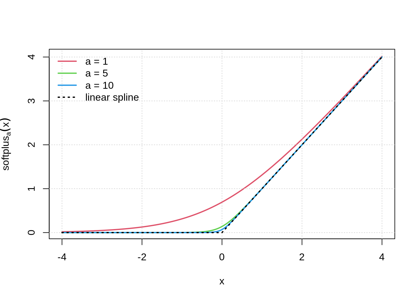

## Poisson regression example with different links
data("FIFA2018", package = "distributions3")
m_exp <- glm(goals ~ difference, data = FIFA2018, family = poisson(link = "log"))
m_splus <- glm(goals ~ difference, data = FIFA2018, family = poisson(link = softplus(1)))
AIC(m_exp, m_splus)

        df      AIC
m_exp    2 359.3942
m_splus  2 359.3774

## comparison of fitted effects
nd <- data.frame(difference = -15:15/10)
nd$mu_exp <- predict(m_exp, newdata = nd, type = "response")
nd$mu_splus <- predict(m_splus, newdata = nd, type = "response")
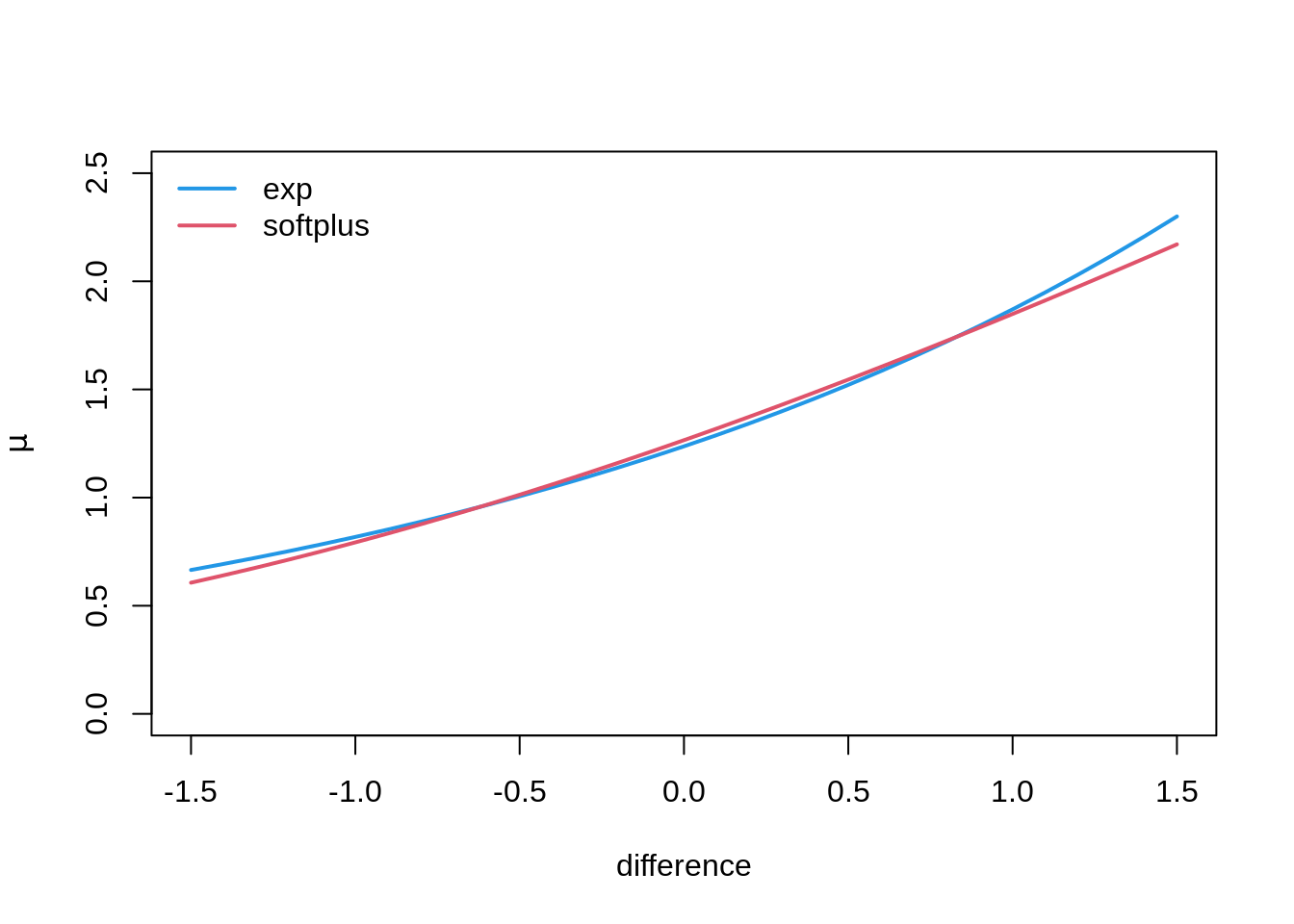
plot(mu_exp ~ difference, data = nd, ylab = expression(mu),
  type = "l", col = 4, lwd = 2, ylim = c(0, 2.5))
lines(mu_splus ~ difference, data = nd, col = 2, lwd = 2)
legend("topleft", c("exp", "softplus"), col = c(4, 2), lwd = 2, lty = 1, bty = "n")