Kumaraswamy Distribution

Description

This function implements the two-parameter Kumaraswamy family for responses in (0, 1).

Usage

## the Kumaraswamy family
Kumaraswamy(a.link = shiftlog, b.link = shiftlog, ...)
KS(a.link = shiftlog, b.link = shiftlog, ...)

## the exp(x) + shift link specification
shiftlog(shift = 1)

Arguments

a.link	Character or function, the link function to be used for parameter a.
b.link	Character or function, the link function to be used for parameter b.
shift	Numeric, the shift parameter to be used for the link.
…	Not used.

Details

The Kumaraswamy distribution is a continuous distribution defined on the interval (0, 1). The probability density function is

\(\displaystyle f(y; a, b) = aby^{a - 1}(1 - y^a)^{b - 1}\)

\(y \in (0, 1)\) is the response, \(a\) and \(b\) are non-negative parameters.

The shiftlog link function is given by:

\(\displaystyle \exp(x) + 1\)

This is the default, since the mode of the distribution is only defined for \(a \geq 1\), \(b \geq 1\).

Value

The family returns an object of class “gamlss2.family”.

Function shiftlog() returns a link specification object of class “link-glm”.

References

Kumaraswamy P (1980). “A Generalized Probability Density Function for Double-Bounded Random Processes.” Journal of Hydrology, 46(1), 79–88. doi:https://doi.org/10.1016/0022-1694(80)90036-0

See Also

gamlss2.family, gamlss2

Examples

library("gamlss2")

## create family object with
## different link specifications
fam <- Kumaraswamy(a.link = shiftlog, b.link = "log")

## simulate data
set.seed(123)
n <- 1000
d <- data.frame("x" = runif(n, -pi, pi))

## true parameters
par <- data.frame(
  "a" = exp(1.2 + sin(d$x)) + 1,
  "b" = 1
)

## sample response
d$y <- fam$r(1, par)

## estimate model using the Kumaraswamy family
m <- gamlss2(y ~ s(x), data = d, family = fam)

GAMLSS-RS iteration  1: Global Deviance = -1504.1261 eps = 0.674808     
GAMLSS-RS iteration  2: Global Deviance = -1504.1299 eps = 0.000002     

## plot estimated effect
plot(m)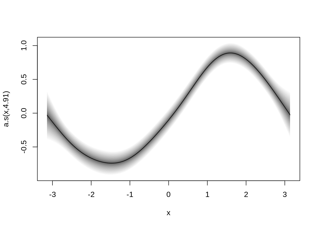

## plot residual diagnostics
plot(m, which = "resid")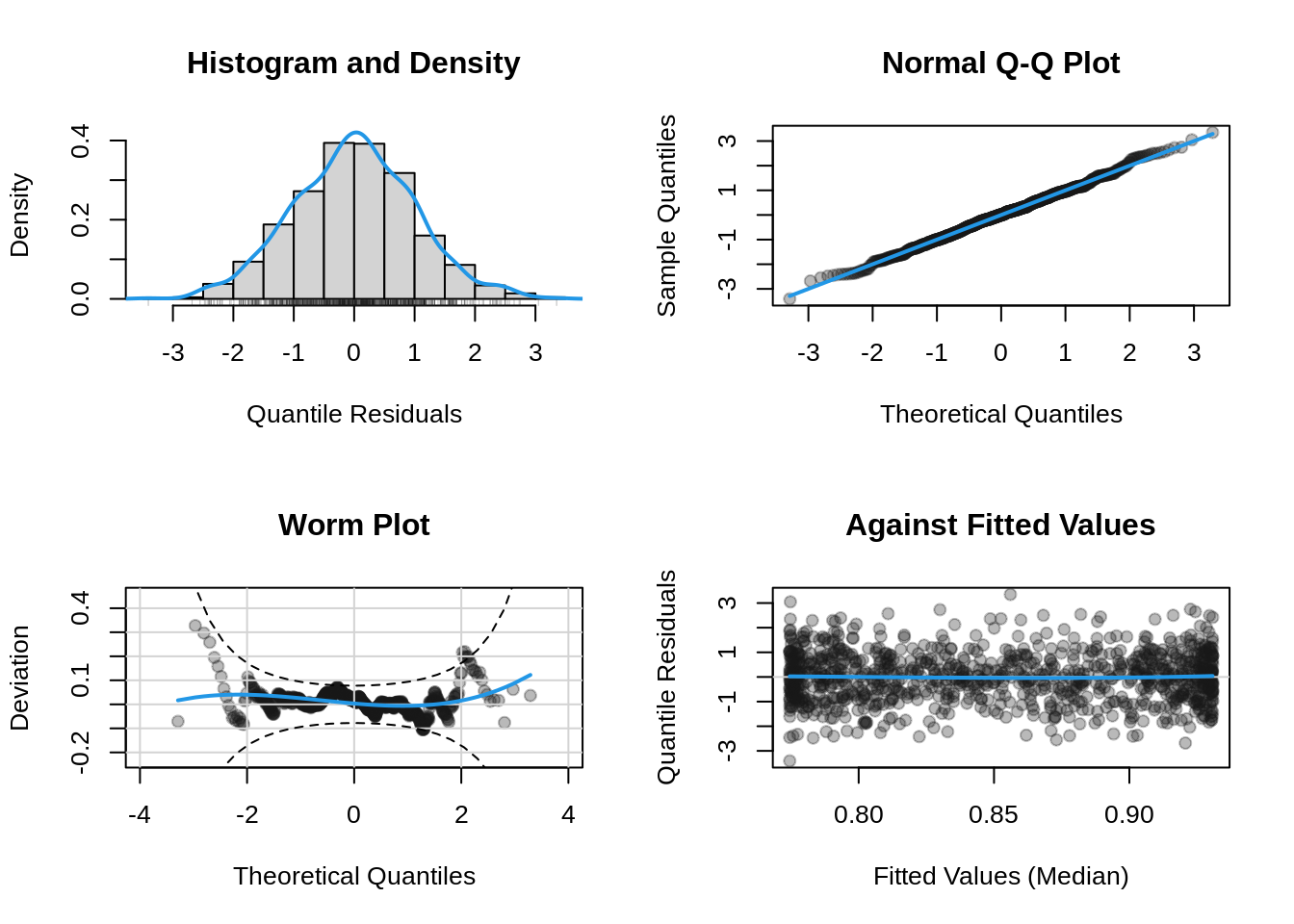

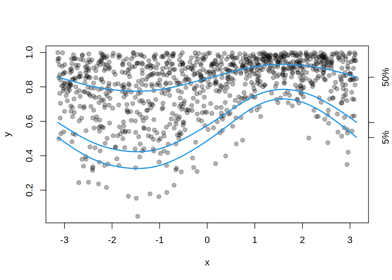
## predict quantiles
p <- quantile(m, probs = c(0.05, 0.1, 0.5))

## plot
plot(d, pch = 19, col = adjustcolor(1, 0.3))
i <- order(d$x)
matlines(d$x[i], p[i, ], lty = 1, col = 4, lwd = 2)
axis(4, at = p[i, ][1, ], labels = names(p))