marginal_predict

Marginal Prediction Profiles for gamlss2 Models

Description

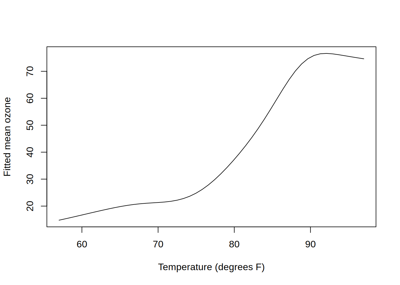
Compute one-variable-at-a-time prediction profiles from a fitted gamlss2 model. Each selected covariate is varied over a grid while the other model covariates are held at representative values.

Usage

marginal_predict(object, newdata = NULL, variables = NULL,
  n = 100L, continuous = median, at = NULL, values = NULL, ...)

Arguments

object A fitted object inheriting from class “gamlss2” or “bamlss2”.

newdata An optional data frame defining the observed ranges, levels, and representative values of the model covariates. By default, the model frame of object is used.

variables A character vector naming the covariates for which profiles should be computed. By default, all covariates used by the model are included.

n A single integer greater than one giving the grid size for numeric, Date, and POSIXct covariates. A covariate that is constant has a one-point grid.

continuous A function, or the name of a function, used to compute the representative value of covariates not currently being varied. The default is median; mean is another common choice. The function must return one value.

at An optional named list specifying values at which covariates should be held fixed. Each element must contain one value.

values An optional named list specifying the prediction grid for one or more of the selected variables.

… Further arguments passed to predict.gamlss2, such as type, model, terms, or se.fit.

Details

For each selected covariate, numeric and date-time covariates are varied over an equally spaced grid spanning their observed range. Factors are varied over their levels, and character and logical covariates over their observed values. The values argument can be used to replace any of these grids.

Covariates not being varied are fixed at at, when supplied. Otherwise, numeric and date-time covariates are summarized by continuous, factors are set to their first level, character variables to their first observed value, and logical variables to FALSE when that value is observed.

Here, marginal prediction means a conditional one-variable profile: predictions are evaluated at one representative combination of the remaining covariates. They are not averages over the empirical joint distribution of those covariates. In models with interactions, the profile is conditional on the interacting covariates’ fixed values; use at to choose scientifically meaningful values.

Value

A named list with one data frame per selected covariate. Each data frame contains the focal covariate followed by the output from predict(object, newdata = …, …). Vector predictions, such as those from type = “response”, are stored in a column named .fit. The representative values computed for the covariates are available in the “fixed” attribute of the returned list. Each is used whenever that covariate is not the focal variable.

Examples

library("gamlss2")

## Same air-quality model as in the first gamlss2() example.
air <- subset(airquality, !is.na(Ozone))
m <- gamlss2(
  Ozone ~ s(Temp) + s(Wind) | s(Temp),
  data = air,
  family = GA
)

GAMLSS-RS iteration  1: Global Deviance = 934.9808 eps = 0.150303     
GAMLSS-RS iteration  2: Global Deviance = 927.3127 eps = 0.008201     
GAMLSS-RS iteration  3: Global Deviance = 924.8517 eps = 0.002653     
GAMLSS-RS iteration  4: Global Deviance = 925.5146 eps = 0.000716     
GAMLSS-RS iteration  5: Global Deviance = 926.9917 eps = 0.001595     
GAMLSS-RS iteration  6: Global Deviance = 928.0621 eps = 0.001154     
GAMLSS-RS iteration  7: Global Deviance = 928.6793 eps = 0.000665     
GAMLSS-RS iteration  8: Global Deviance = 928.9916 eps = 0.000336     
GAMLSS-RS iteration  9: Global Deviance = 929.1382 eps = 0.000157     
GAMLSS-RS iteration 10: Global Deviance = 929.2117 eps = 0.000079     
GAMLSS-RS iteration 11: Global Deviance = 929.2443 eps = 0.000035     
GAMLSS-RS iteration 12: Global Deviance = 929.2588 eps = 0.000015     
GAMLSS-RS iteration 13: Global Deviance = 929.2643 eps = 0.000005

## Conditional mean profiles for temperature and wind.
mp <- marginal_predict(
  m,
  variables = c("Temp", "Wind"),
  n = 50,
  type = "response"
)
head(mp$Temp)

      Temp     .fit
1 57.00000 14.77474
2 57.81633 15.28238
3 58.63265 15.80438
4 59.44898 16.33702
5 60.26531 16.87571
6 61.08163 17.41530

attr(mp, "fixed")

$Temp
[1] 79

$Wind
[1] 9.7

plot(.fit ~ Temp, data = mp$Temp, type = "l",
  xlab = "Temperature (degrees F)", ylab = "Fitted mean ozone")

## Supply a custom grid and condition on a particular wind speed.
mp2 <- marginal_predict(
  m,
  variables = "Temp",
  values = list(Temp = seq(60, 95, by = 5)),
  at = list(Wind = 5),
  type = "response"
)
mp2$Temp

  Temp     .fit
1   60 20.54507
2   65 24.36994
3   70 26.24466
4   75 30.54225
5   80 45.91176
6   85 70.11447
7   90 92.58613
8   95 92.93267