Residuals for GAMLSS Models

Description

Extracts residuals from fitted gamlss2 objects. By default, normalized quantile residuals are returned. Response residuals can be obtained as observed responses minus fitted distribution means. A plotting method for residual diagnostic plots is also provided.

Usage

## S3 method for class 'gamlss2'
residuals(object,
  type = c("quantile", "response", "parameter"), newdata = NULL, ...)

## S3 method for class 'gamlss2.residuals'
plot(x, which = NULL, spar = TRUE, ...)

Arguments

object An object of class “gamlss2”.
type Character specifying the type of residuals to be computed. The default “quantile” computes normalized quantile residuals. “response” computes observed responses minus fitted distribution means. “parameter” is reserved for parameter-specific residuals and is currently not implemented.
newdata An optional data frame in which to evaluate the residuals. If omitted, residuals are evaluated for the data used to fit the model. When supplied, newdata must also contain the response variable.
Additional arguments passed on to methods, family-specific residual functions, or predict.gamlss2.
x An object of class “gamlss2.residuals”, typically produced by residuals.gamlss2.
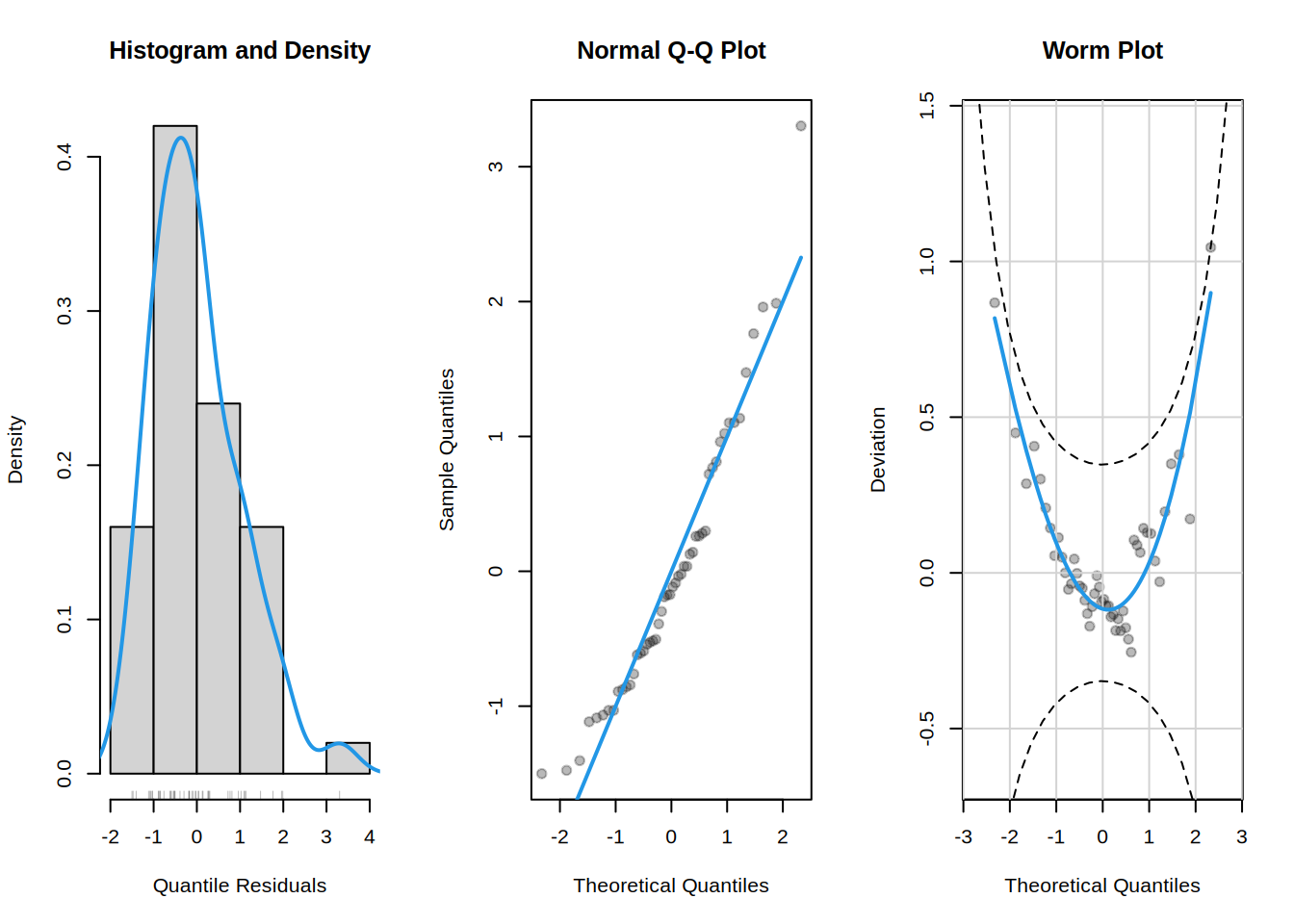
which Character or integer selecting the diagnostic plot(s). Available plots are “hist-resid” for a histogram with kernel density estimate, “qq-resid” for a normal quantile-quantile plot, and “wp-resid” for a worm plot. If omitted, all three plots are produced. Integers 1, 2, and 3 select these plots in the same order.
spar Logical. Should graphical parameters be set automatically for multiple plots?

Details

Normalized quantile residuals are obtained by evaluating the fitted distribution function at the observed responses and transforming the resulting probabilities to the standard normal scale. For continuous response distributions this is

\(r_i = \Phi^{-1}\{F(y_i | \hat\theta_i)\},\)

where \(F()\) is the fitted cumulative distribution function and \(\hat\theta_i\) denotes the fitted distribution parameters for observation \(i\).

For discrete response distributions, randomized quantile residuals are used: a uniform random probability is drawn between the fitted distribution probabilities just below and at the observed response before applying the standard normal quantile function. Thus, repeated calls may differ for discrete families unless the random-number seed is fixed.

If the family object supplies a family-specific residual function, this is used. Otherwise, quantile residuals are computed from the family cumulative distribution function. If no cumulative distribution function is available, the function falls back to response residuals and issues a warning.

Response residuals are computed as

\(y_i - \mu(\hat\theta_i),\)

where \(\mu()\) is the family mean function if available. Otherwise the first distribution parameter is used as the fitted mean.

Non-finite residuals are replaced by NA. The plotting method provides simple residual diagnostics for checking whether quantile residuals are approximately standard normal.
Value

A numeric vector of residuals with class “gamlss2.residuals” and an attribute “type” indicating the residual type. The plotting method is called for its side effect and returns NULL invisibly.

References

Dunn PK, Smyth GK (1996). “Randomized Quantile Residuals.” Journal of Computational and Graphical Statistics, 5(3), 236–244. doi:10.1080/10618600.1996.10474708

See Also

gamlss2, predict.gamlss2, plot.gamlss2

Examples

library("gamlss2")

## data
data("cars", package = "datasets")

## fit heteroscedastic normal GAMLSS model
m <- gamlss2(dist ~ s(speed) | s(speed), data = cars, family = NO)
GAMLSS-RS iteration  1: Global Deviance = 405.4242 eps = 0.129640     
GAMLSS-RS iteration  2: Global Deviance = 405.2294 eps = 0.000480     
GAMLSS-RS iteration  3: Global Deviance = 405.2069 eps = 0.000055     
GAMLSS-RS iteration  4: Global Deviance = 405.1868 eps = 0.000049     
GAMLSS-RS iteration  5: Global Deviance = 405.17 eps = 0.000041     
GAMLSS-RS iteration  6: Global Deviance = 405.1562 eps = 0.000033     
GAMLSS-RS iteration  7: Global Deviance = 405.1452 eps = 0.000027     
GAMLSS-RS iteration  8: Global Deviance = 405.1365 eps = 0.000021     
GAMLSS-RS iteration  9: Global Deviance = 405.1297 eps = 0.000016     
GAMLSS-RS iteration 10: Global Deviance = 405.1244 eps = 0.000012     
GAMLSS-RS iteration 11: Global Deviance = 405.1206 eps = 0.000009     
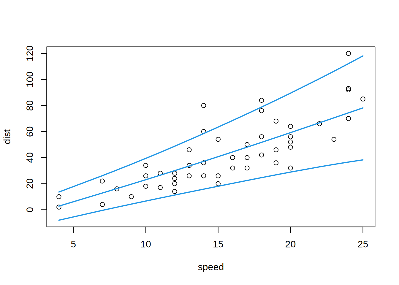
## plot estimated quantiles
p <- quantile(m, probs = c(0.05, 0.5, 0.95))
plot(dist ~ speed, data = cars, ylim = range(cars$dist, p))
matlines(cars$speed, p, lty = 1, col = 4, lwd = 2)

## normalized quantile residuals
rq <- residuals(m)
summary(rq)
     Min.   1st Qu.    Median      Mean   3rd Qu.      Max. 
-1.500618 -0.725769 -0.144190  0.004394  0.615212  3.302438 
attr(rq, "type")
[1] "quantile"
## response residuals
rr <- residuals(m, type = "response")
summary(rr)
    Min.  1st Qu.   Median     Mean  3rd Qu.     Max. 
-27.1865  -9.5648  -1.5637   0.4061   7.1394  45.6459 
## residuals for new data
nd <- cars[1:10, ]
residuals(m, newdata = nd)
          1           2           3           4           5           6 
-0.11542272  1.10117234 -1.08708247  1.13528030 -0.02127194 -1.03123936 
          7           8           9          10 
-0.50444369  0.29901487  1.10247343 -0.89074902 
attr(,"type")
[1] "quantile"
attr(,"class")
[1] "gamlss2.residuals" "numeric"          
## diagnostic plots
plot(rq)

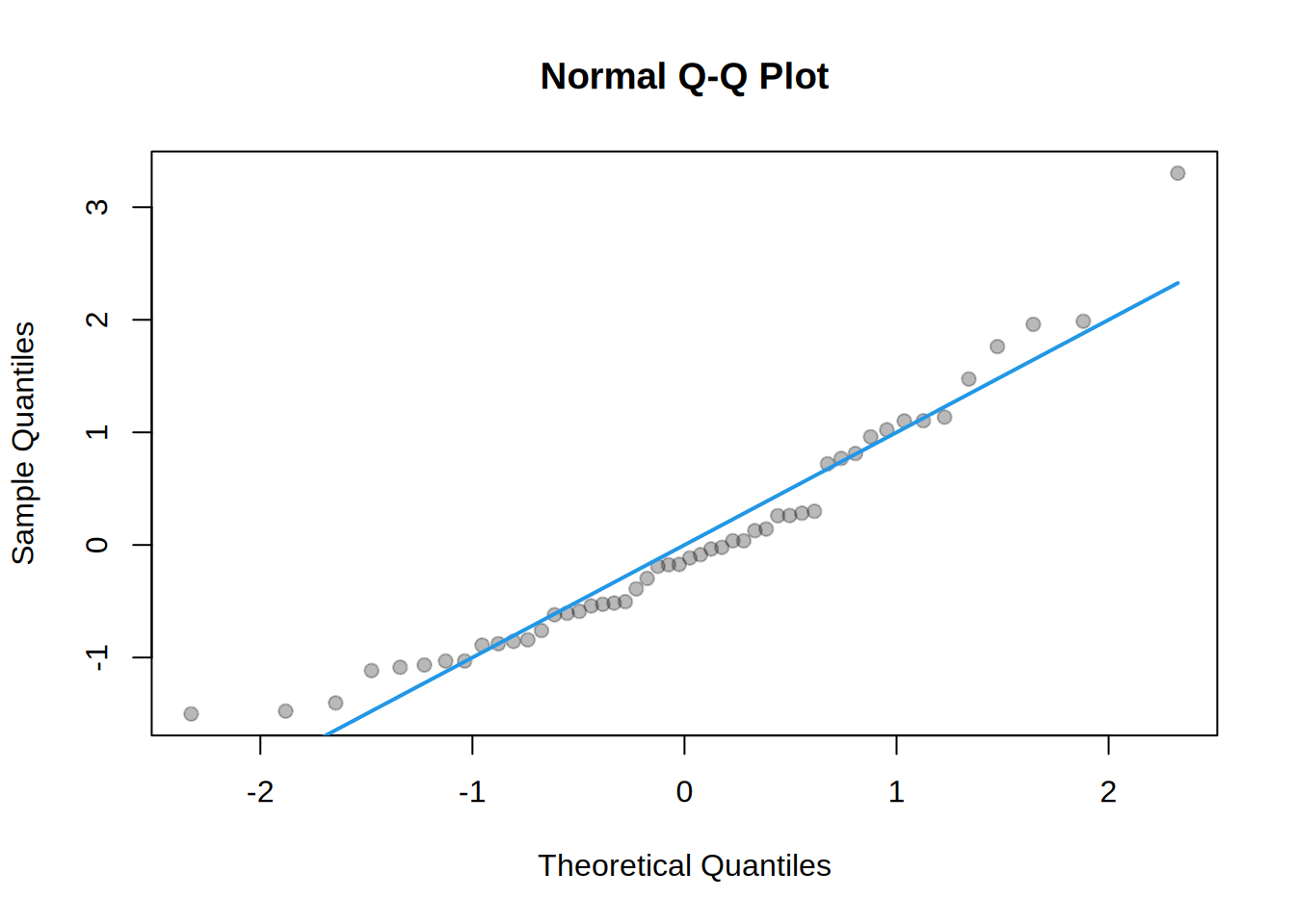
plot(rq, which = "qq-resid")