Model Selection

A distribution regression model is defined as

\[\begin{split} y_i & \stackrel{\small{ind}}{\sim }& \mathcal{D}( \theta_{1i}, \ldots, \theta_{ki}) \nonumber \\ g(\theta_{1i}) &=& b_{10} + s_1({x}_{1i}) + \ldots, s_p({x}_{pi}) \nonumber\\ \ldots &=& \ldots \nonumber\\ g({\theta}_{ki}) &=& b_0 + s_1({x}_{1i}) + \ldots, s_p({x}_{pi}) \end{split} \tag{1}\] where \(\mathcal{D}( )\) is the assumed distribution which depends on parameters \(\theta_{1i}, \ldots, \theta_{ki}\) and where all the parameters can be functions of the explanatory variables \(({x}_{1i}, \ldots, {x}_{pi})\). In reality we do not know the distribution \(\mathcal{D}( )\) and also we do not know which and how the variables \(({x}_{1i}, \ldots, {x}_{pi})\) effect the parameters \(\theta_{1i}, \ldots, \theta_{ki}\). So the model selection in a distributional regression model should have the following steps;

select the best fitting distribution and,
select the relevant variables for the parameters and how they effect the parameters.

One way to achieve that is the following general algorithm for searching for best model;

step 0: Defining a set of appropriate distributions for the response \(\mathcal{D}_J()\) for \(j=1,\ldots, J,\) see section Section 1.1 how to do that,
step 1: FOR \(J\) in \(j=1,\ldots, J\)
step 2: use distribution \(\mathcal{D}_J()\) to SELECT the appropriate variables \(({x}_{1i}, \ldots, {x}_{pi}).\)
step 3: END the loop
step 4: SELECT the distribution \(\hat{\mathcal{D}}_J()\) and variables which give a minimum values for a selection criterion measure.

The selection criterion could be a GAIC defined on the training data or a measure defined on the test, out of bag, data. While the above algorithm could work reasonable with data having a relative small number or explanatory variables could be very slow for data with a large number of explanatory variables.

Cutting corners could improve the speed of the algorithm. For example, if the practitioner gives up the smooth additive structure, that gamlss2 provides, and he/she prepare to use only linear terms, a LASSO method can be used at step 2 which will speed up things. Also if the practitioner has confidence on a particular distribution choice, then only the selection step 2 could be performed. The support for a specific distribution can be enforced my the preliminary analysis for choosing a distribution described in Section 1.2 and suggested in Stasinopoulos et al. (2024).

1 Select a distribution

1.1 The range of the response

The first thing to take into the account in the selection of the distribution is the range of the response variable, that is, the distribution should be defined in right range. Figure 1 shows the different possibilities depending on whether the response is continuous, discrete of factor If the response is continuous and has negative values a distribution in the real line is appropriate. For positive responses a positive real line distribution is appropriate. For bounded continuous response we have the options;

to use a distributions in the range between 0 and 1, i.e. the beta distribution see Chapter 21 of Rigby et al. (2019);
to transform a continuous distribution with range \((-\infty, \infty)\) to a range \((0,1)\) using the logit transformation see Section 13.2.2 of Rigby et al. (2019);
to create an appropriate truncated distribution which takes values \((0,1)\) see Section 13.7 of Rigby et al. (2019); or
to create a generalised Tobit distribution using censoring. This methodology is also appropriate for inflated distributions see Chapter 9 of Rigby et al. (2019).

For count response the only consideration is whether the counts are finite or not. For infinite counts a discrete distribution similar to the Poisson distribution can be used. For finite counts a discrete distribution like the binomial can be used. The case in which the response is a categorical variable (taht is a factor) is called classification regression. If the factor is an ordered factor appropriate models, ordinal regression models, exist but we will not deal with them here. For unordered factor responses a binomial distribution can be use if the classification is binary otherwise a multinomial distribution if the resposnse has more than two categories. Note that for classification problems, there is a vast literature in machine learning to deal with the problem.

flowchart LR
  A[responce] --> B(continuous) 
  A --> C[discrete]
  A --> D[factor]
  B --> F[real line]
  B --> G[pos. real line]
  B --> H[0 to 1]
  C --> J[infinite count]
  C --> I[finite count]
  D --> K[unordered]
  D --> L[ordered]
  I --> N[binary]
  K --> N[binary]

Figure 1: The response determines which type of distribution to use.

1.2 Preliminary analysis

A preliminary analysis in selecting the distribution can be performed using the chooseDist() function of the package gamlss. Here we used the rent data of the package gamlss.data. We first bring the package and the data set in;

library(gamlss2)
library(gamlss)
da <- rent99[, -c(2,9)]
head(da)

      rent area yearc location bath kitchen cheating
1 109.9487   26  1918        2    0       0        0
2 243.2820   28  1918        2    0       0        1
3 261.6410   30  1918        1    0       0        1
4 106.4103   30  1918        2    0       0        0
5 133.3846   30  1918        2    0       0        1
6 339.0256   30  1918        2    0       0        1

The response variable is is rent and there are two continuous, the area of the flat area and the year of construction yearc and 4 categorical variables, location, bath, kitchen and central heating, cheating.

Here, first we fit a linear model with all explanatory variables to the location parameters \(\mu\) and scale parameter \(\sigma\). Later we use the function chooseDist() to find out which distribution from the ones in positive real line fit, type="realplus", best fit the data, given that \(\mu\) and \(\sigma\) models are fitted linearly with all available variables. Note that, in order to speed up the procedure, we used here a parallel version of chooseDist() using snow with 10 NCPUS (the maximum that our machine can take). Please modify accordantly to your machine capabilities.

 m1 <- gamlss2(rent~.|., data=da, family=GA,trace=FALSE)
 M1 <- gamlss:::chooseDist(m1, type="realplus", parallel="snow", ncpus=10)

minimum GAIC(k= 2 ) family: BCTo 
minimum GAIC(k= 3.84 ) family: BCCGo 
minimum GAIC(k= 8.03 ) family: BCCGo

The function chooseDist() chooses the “best” distribution according to a GAIC criterion. In our case the BCTo distribution was chosen using AIC while the BCCGo using \(\chi^2\) or BIC criteria, respectively.

2 Select appropriate variables

The methodology of “which explanatory variable is needed and for which parameters” depends on the scope of modelling, while special attention has to be taken for non-linear relationships and for interaction. If the scope of the model is to provide good interpretation then the additive smooth structure of gamlss2is adequate because can cope well with non-linearities and relatively well with interactions. Note that interactions in an additive structure have to specified explicitly while in some machine learning algorithms like neural network they come as part of the model. Machine learning algorithms like random forest and neural networks are more difficult to interpreter therefore more suited for prediction purposes. Here we will discuss the the step-wise methodology while boosting is discussed in a different vignette?.

data("rent", package = "gamlss.data")

Because the possiblility of linear interactions, we shall scale the two continuous covariates first;

rent$Fl <- scale(rent$Fl)
rent$A <- scale(rent$A)

The formula defines the searching scope of the search;

f <- R ~ Fl + A + Fl:A + loc + s(Fl) + s(A) + te(Fl, A) |
  Fl + A + loc + Fl:A + s(Fl) + s(A) + te(Fl, A)

Here we use the the stepwise algorithm to find the “best” explanatory variables using a Gamma family model;

b <- step_gamlss2(f, data = rent, family = GA, K = 2)

Bidirectional Linear Selection
  GAIC = 28104.4252 <+> parameter mu, term Fl
  GAIC = 27996.2040 <+> parameter mu, term A
  GAIC = 27937.8423 <+> parameter sigma, term A
  GAIC = 27905.5919 <+> parameter mu, term loc3
  GAIC = 27863.1707 <+> parameter mu, term loc2
  GAIC = 27860.8491 <+> parameter sigma, term loc3
  GAIC = 27856.2102 <+> parameter sigma, term loc2
Bidirectional Selection
  GAIC = 27768.8887 <+> parameter mu, term te(Fl,A)
  GAIC = 27766.8886 <-> parameter mu, term Fl
  GAIC = 27748.6682 <+> parameter sigma, term s(A)
  GAIC = 27746.7130 <-> parameter mu, term A
Continue
Final Model
$mu
.. ~1 + loc3 + loc2 + te(Fl, A)
$sigma
.. ~1 + A + loc3 + loc2 + s(A)

Note that step_gamlss2() is equivalent to using

b <- gamlss2(f, data = rent, family = GA, optimizer = stepwise, K = 2)

The new_formula() function will show the new selected model terms;

new_formula(b)

$mu
R ~ loc3 + loc2 + te(Fl, A)

$sigma
~1 + A + loc3 + loc2 + s(A)

Here is the summary of the final model;

summary(b)

Call:
gamlss2(formula = formula, data = ..1, family = ..2, ... = pairlist(optimizer = stepwise, K = K, strategy = strategy, keeporder = keeporder, cores = cores))
---
Family: GA 
Link function: mu = log, sigma = log
*--------
Parameter: mu 
---
Coefficients:
            Estimate Std. Error t value Pr(>|t|)    
(Intercept)  6.44057    0.03170 203.171  < 2e-16 ***
loc3         0.31100    0.03475   8.950  < 2e-16 ***
loc2         0.21511    0.03334   6.452 1.39e-10 ***
---
Smooth terms:
    te(Fl,A)
edf     9.51
*--------
Parameter: sigma 
---
Coefficients:
            Estimate Std. Error t value Pr(>|t|)    
(Intercept) -0.86451    0.04454 -19.410  < 2e-16 ***
A           -0.14138    0.01388 -10.186  < 2e-16 ***
loc3        -0.19338    0.04989  -3.876  0.00011 ***
loc2        -0.12580    0.04746  -2.651  0.00810 ** 
---
Signif. codes:  0 '***' 0.001 '**' 0.01 '*' 0.05 '.' 0.1 ' ' 1
---
Smooth terms:
      s(A)
edf 4.8959
*--------
n = 1969 df =  21.41 res.df =  1947.59
Deviance = 27703.9013 Null Dev. Red. = 3.17%
AIC = 27746.713 elapsed = 19.84sec

and here are the smooth fitted plots;

plot(b)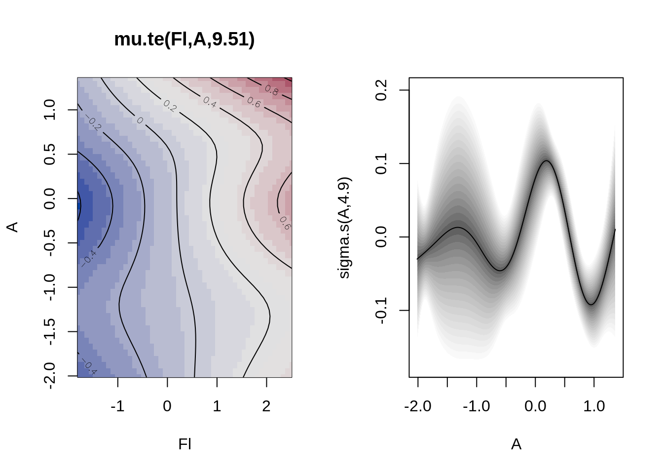

To get the diagnostic plots of the model use;

plot(b, which = "resid")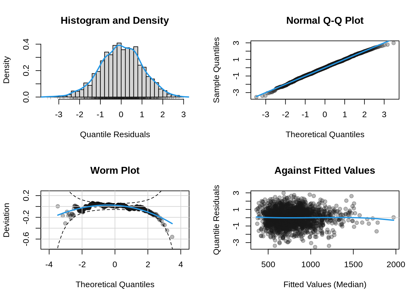

The selection path can be plotted using;

plot(b, which = "selection")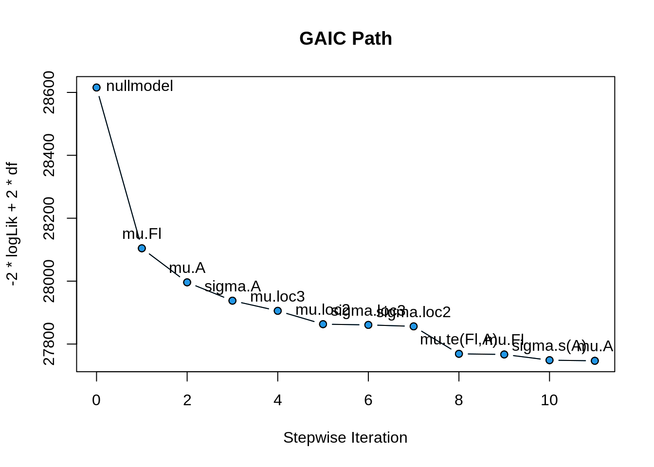

Now we use a more complex diatributional model using the BCTo family. First we define the formula.

f <- R ~ Fl + A + Fl:A + loc + s(Fl) + s(A) + te(Fl, A) |
  Fl + A + loc + Fl:A + s(Fl) + s(A) + te(Fl, A) |
  Fl + A + loc + Fl:A + s(Fl) + s(A) + te(Fl, A) |
  Fl + A + loc + Fl:A + s(Fl) + s(A) + te(Fl, A)

Note

Note that if modelling of certain parameters is not required the formula 1| could be used.

Next we use the function step_gamlss2() but using different options this time, more specificaly we use;

K=log(3082) so the criterion used will be BIC rather than AIC and therefore less terms will be allowed in the model.
strategy = c("forward.linear", "both") so specified explicitly which strategies should be used, see the hlp file for more startegies.

b <- step_gamlss2(f, data = rent, family = BCTo,
  K = log(3082), strategy = c("forward.linear", "both"),
  keeporder = TRUE)

Forward Linear Selection
  GAIC = 28121.0230 <+> parameter mu, term Fl
  GAIC = 28028.2802 <+> parameter mu, term A
  GAIC = 28001.2470 <+> parameter mu, term loc3
  GAIC = 27947.0011 <+> parameter sigma, term A
  GAIC = 27936.1483 <+> parameter nu, term A
Bidirectional Selection
  GAIC = 27894.8174 <+> parameter mu, term s(A)
  GAIC = 27857.4438 <+> parameter mu, term loc2
  GAIC = 27849.3901 <-> parameter mu, term A
Continue
Final Model
$mu
.. ~1 + Fl + loc3 + loc2 + s(A)
$sigma
.. ~1 + A
$nu
.. ~1 + A
$tau
.. ~1

The final model model seems lot simpler than the one obtain using AIC and the GA distribution. Let us looks at its residual diagnostic plots.

plot(b, which = "resid")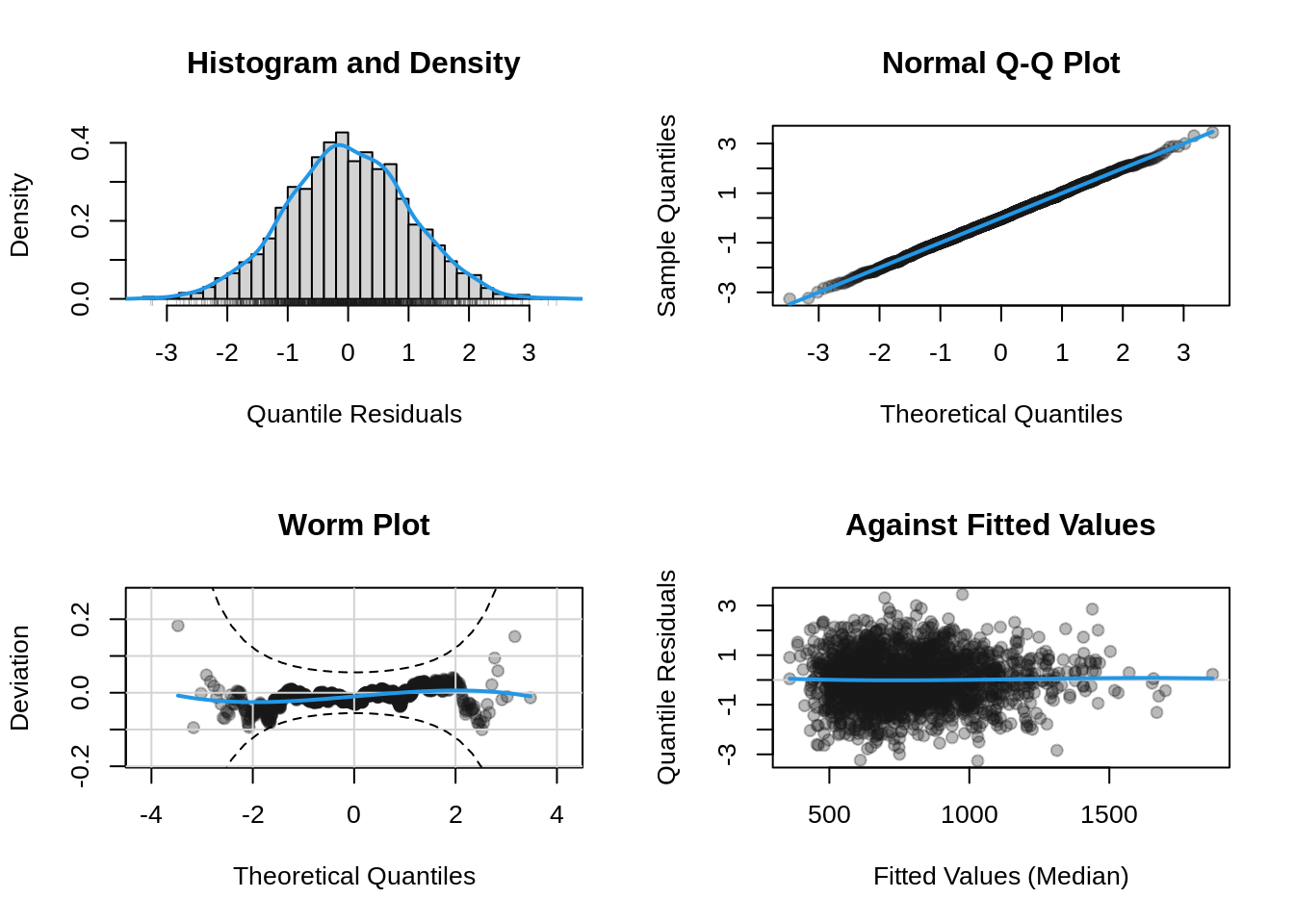

The residual plots lok goog. Next we plot the path of selection.

plot(b, which = "selection")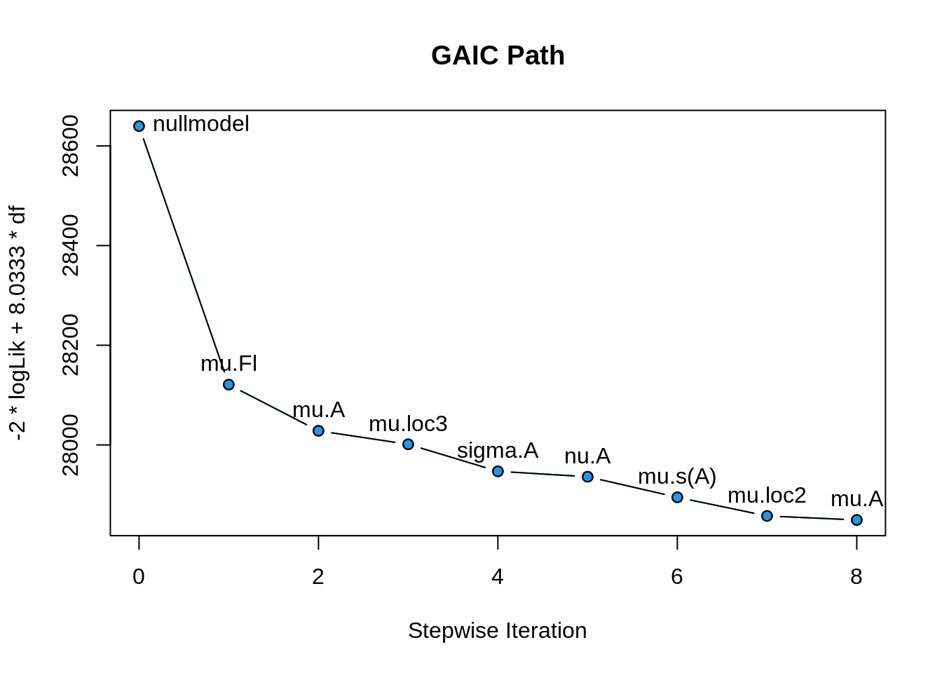

3 Conclusions

Selection in any distributional regression model like gamlss2 requires both the selection of the distribution and also the selection of the expanatory of variables affecting the parameters of the distribution. A general procedure is proposed here but not implemented. Mikis we should do that. We have shown how distibutions and variables can be sellected seperately.

References

Rigby, R. A., and D. M. Stasinopoulos. 2005. “Generalized Additive Models for Location, Scale and Shape.” Journal of the Royal Statistical Society C 54 (3): 507–54. https://doi.org/10.1111/j.1467-9876.2005.00510.x.

Rigby, R. A., D. M. Stasinopoulos, G. Z. Heller, and F. De Bastiani. 2019. Distributions for Modeling Location, Scale, and Shape: Using GAMLSS in R. Boca Raton: Chapman & Hall/CRC. https://doi.org/10.1201/9780429298547.

Stasinopoulos, M. D., T. Kneib, N. Klein, A. Mayr, and G. Z Heller. 2024. Generalized Additive Models for Location, Scale and Shape: A Distributional Regression Approach, with Applications. Vol. 56. Cambridge University Press. https://doi.org/10.1017/9781009410076.